 Scientify
About this page
Tutorial- What this page solves
- You need a band structure from QE, but you are unsure how to set the parameters, how to tell whether the gap is direct or indirect, and how far your result may differ from the literature.
- Who it is for
- Graduate students in materials science, physics or chemistry using QE for the first time. You should be comfortable with the Linux command line and know what the Brillouin zone and k-points are.
- What you will have
- You can run every monolayer MoS2 calculation here and apply the same workflow to your own 2D material.
- Covers
- Input files for scf, structure optimization, bands and DOS of monolayer MoS2
- Convergence results for cutoffs, k-points and vacuum
- A script that identifies direct and indirect gaps
- What to change for SOC and how to read the splitting at K
- Bulk MoS2 and the effect of D3 dispersion
- Comparison with published and experimental values
- Does not cover
- Compiling and installing QE
- GW and BSE calculations
- Phonons and optical properties
Main steps
Step 1
Why this stepA QE input needs the cell, the atomic coordinates and the pseudopotential file names. This step settles those three items.
Monolayer MoS2 has space group P-6m2, with one Mo and two S atoms in the primitive cell. The cell height c is 15 Å here, so vacuum separates the periodic images. The scf input below already contains the optimized structure.
The pseudopotentials come from SSSP 1.3.0 PBE efficiency: an SG15 ONCV file for Mo and a GBRV 1.4 ultrasoft file for S. Mo and S contribute 14 and 6 valence electrons, which gives 26 electrons per cell. Without SOC each band holds 2 electrons, so 13 bands are occupied. nbnd=18 adds 5 empty bands.
ATOMIC_POSITIONS crystal means fractional coordinates. The in-plane lattice vectors here are 120° apart, and this convention determines the coordinates of K later on.
&CONTROL
 calculation='scf', prefix='mos2', pseudo_dir='./pseudo',
 outdir='./tmp', tprnfor=.true., tstress=.true., verbosity='high',
/
&SYSTEM
 ibrav=0, nat=3, ntyp=2, ecutwfc=55, ecutrho=440, nbnd=18, occupations='fixed',
/
&ELECTRONS
 conv_thr=1d-9, mixing_beta=0.4, diagonalization='david',
/
ATOMIC_SPECIES
Mo 95.95 Mo_ONCV_PBE-1.0.oncvpsp.upf
S 32.06 s_pbe_v1.4.uspp.F.UPF
CELL_PARAMETERS angstrom
3.1837669586084907 0 0
-1.5918834793042453 2.7572230658844723 0
0 0 14.999999999999998
ATOMIC_POSITIONS crystal
Mo 0 0 0.5
S 0.333333333333 0.666666666667 0.6042046659769958
S 0.333333333333 0.666666666667 0.39579533402300415
K_POINTS automatic
12 12 1 0 0 0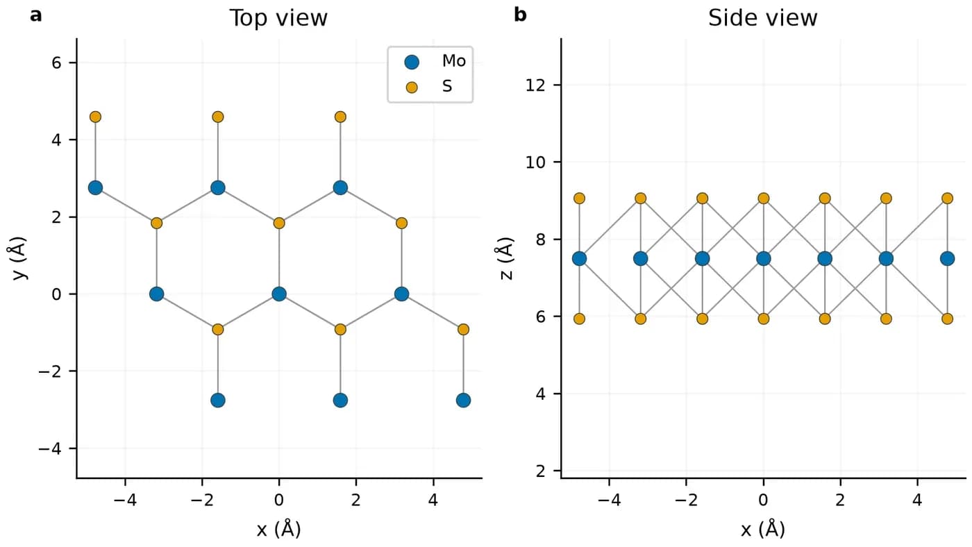
Step 2
Why this stepThese parameters set the numerical error. Change one at a time and keep the others fixed.
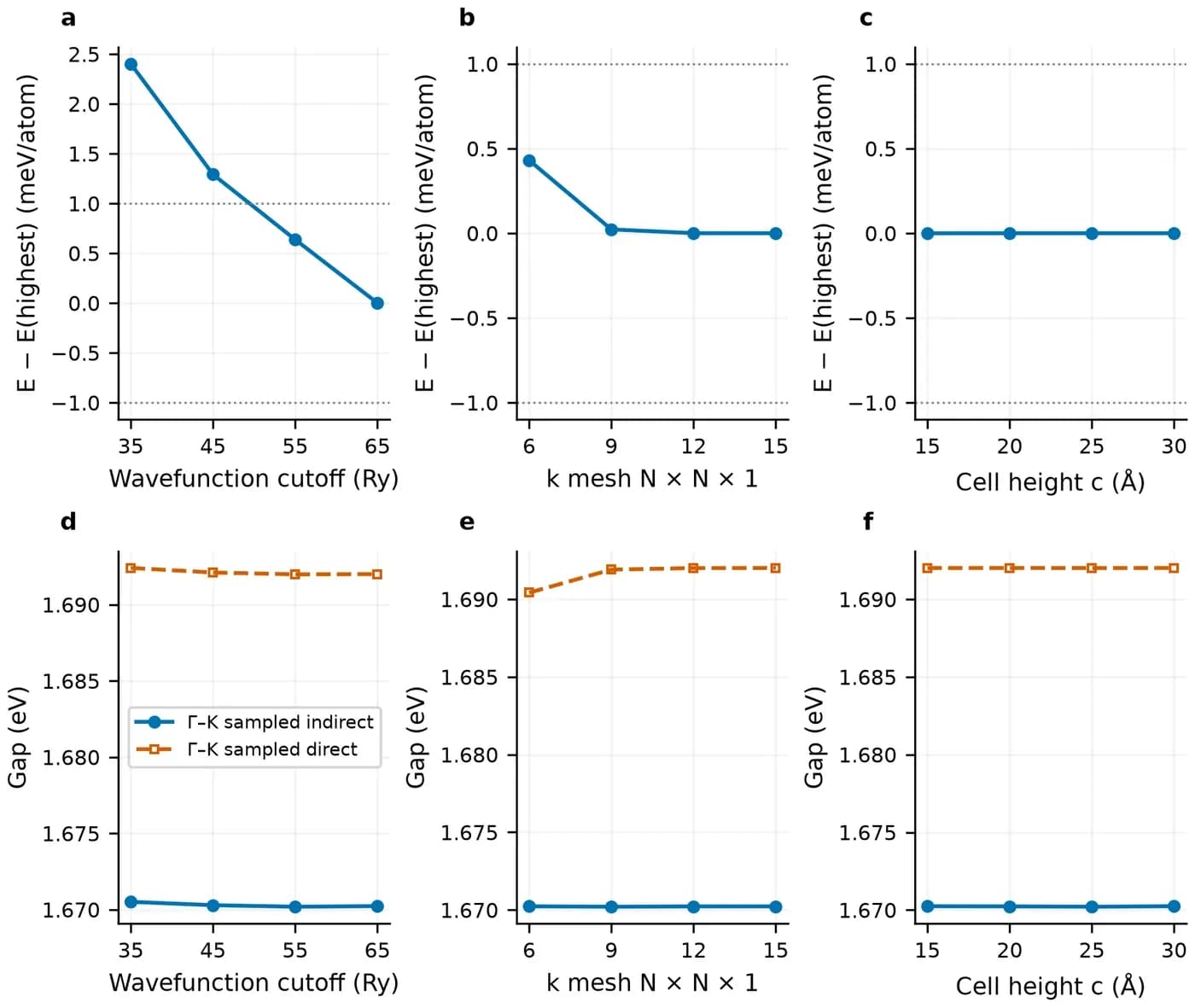
Set the criteria before looking at results. The criteria here are a total-energy change below 1 meV/atom and a gap change below 10 meV between neighbouring values. The SSSP recommendation for these pseudopotentials is ecutwfc 35 Ry and ecutrho 280 Ry, which is only a starting point. In this test 35 Ry is 2.40 meV/atom above 65 Ry and 45 Ry is 1.29 meV/atom above it. Both exceed 1 meV, so 55 Ry was chosen.
Test ecutrho separately. The main scan keeps ecutrho at 8 times ecutwfc, which cannot separate the two errors. A second scan fixes ecutwfc at 55 Ry and tests 330, 440, 550 and 660 Ry. The total energies at 440 and 660 Ry differ by 0.008 meV/atom.
The gap converges faster than the total energy in this system. From 55 to 65 Ry the energy changes by 0.64 meV/atom and the indirect gap by 0.04 meV. Watching only the gap can stop the test too early, and structure optimization also needs the energy and forces to be converged.
| Parameter | Values tested | Chosen | Change at the chosen value |
|---|---|---|---|
| ecutwfc (ecutrho = 8×) | 35, 45, 55, 65 Ry | 55/440 Ry | Against 65 Ry: energy 0.64 meV/atom, indirect gap 0.04 meV |
| ecutrho (ecutwfc = 55 Ry) | 330, 440, 550, 660 Ry | 440 Ry | Against 660 Ry: energy 0.008 meV/atom, indirect gap 0.02 meV |
| k mesh N×N×1 | 6, 9, 12, 15 | 12×12×1 | k6 already meets the criteria against denser meshes (at most 0.43 meV/atom and 1.59 meV); 12 was chosen for more stable forces during optimization |
| Cell height c | 15, 20, 25, 30 Å | 15 Å | Against taller cells: at most 0.0001 meV/atom and 0.03 meV |
| Fully relativistic ecutwfc (ecutrho = 4×) | 35 to 95 Ry in 10 Ry steps | 95/380 Ry | 85→95 Ry: energy 0.18 meV/atom |
Step 3
Why this stepBring the lattice constant and atomic positions to equilibrium while keeping the vacuum thickness fixed.
Use calculation='vc-relax' and set cell_dofree='2Dxy' in &CELL. The cell then changes only in plane and c stays at 15 Å. calculation='relax' moves atoms only and cannot give the equilibrium lattice constant.
The optimization starts from a = 3.18 Å, with a force threshold of 1×10⁻⁴ Ry/bohr and an in-plane stress threshold of 0.1 kbar. The result is a = 3.18377 Å, an Mo–S bond of 2.41288 Å and an S–S distance of 3.12614 Å across the layer.
&CONTROL
 calculation='vc-relax', forc_conv_thr=1d-4, etot_conv_thr=1d-6,
/
&IONS
 ion_dynamics='bfgs'
/
&CELL
 cell_dynamics='bfgs', cell_dofree='2Dxy', press_conv_thr=0.1
/Step 4
Why this stepThe bands run reads the scf charge density and computes eigenvalues along the chosen path.
Run scf on the optimized structure first. The bands input keeps the structure, pseudopotentials, cutoffs, prefix and outdir, and changes only calculation and K_POINTS.
With K_POINTS crystal_b, the first line is the number of path nodes. Each following line gives fractional reciprocal coordinates and the number of points to the next node. The integer on the last line has no effect but cannot be omitted. With 120° lattice vectors, M is (1/2, 0, 0) and K is (1/3, 1/3, 0). A different lattice convention changes the fractional coordinates of K, so check them against your own vectors.
bands.x only post-processes: it writes the pw.x eigenvalues to path.dat. The energy zero has no physical meaning, so subtract the valence band maximum when plotting.
&CONTROL
 calculation='bands',
/
K_POINTS crystal_b
4
0 0 0 35
0.5 0 0 35
0.333333333333 0.333333333333 0 35
0 0 0 1&BANDS
prefix='mos2', outdir='./tmp', filband='path.dat', lsym=.false.
/pw.x -in 02-scf.in > 02-scf.out
pw.x -in 03-bands.in > 03-bands.out
bands.x -in 04-bandsx.in > 04-bandsx.outStep 5
Why this stepValence maxima a few tens of meV apart are hard to distinguish on a plot, so the assignment has to be numerical.
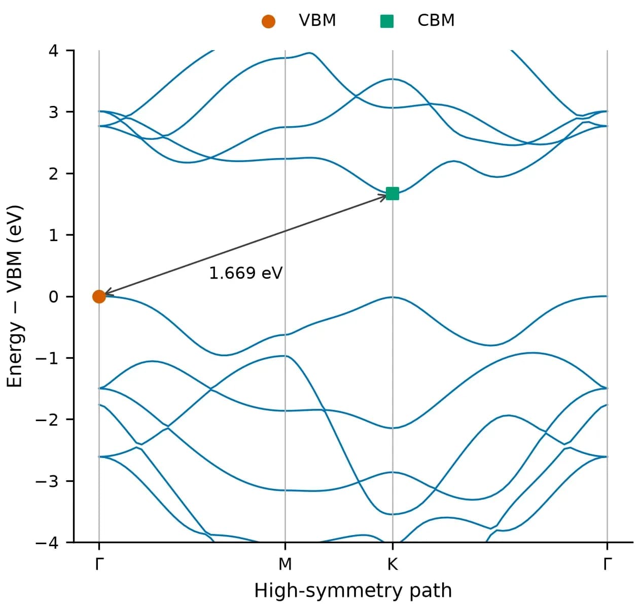
At each k-point, take band 13 as the valence energy Ev(k) and band 14 as the conduction energy Ec(k). The fundamental gap is the minimum of Ec over all k minus the maximum of Ev over all k. The smallest direct gap is the minimum of Ec−Ev at each k. If the two numbers are equal the gap is direct, otherwise it is indirect.
The script below applies this definition. The k coordinates it prints are the Cartesian values written by bands.x in units of 2π/a, so K appears as (0.333, 0.577, 0).
A high-symmetry path does not prove that the global edges were found. A 24×24×1 uniform mesh was used as a check here. Its fundamental gap differs from the path value by 0.07 meV, and the edges stay at Γ and K.
bands.x keeps only three decimals. For differences below 1 meV, read the eigenvalues from the XML files in outdir. The five-decimal values in the tables on this page come from XML.
#!/usr/bin/env python3
"""从 bands.x 的 filband 文件读出价带顶、导带底和带隙。
用法:python3 band_edges.py path.dat 13
第二个参数是占据带数:不开 SOC 时单层 MoS2 为 13,开 SOC 时为 26。"""
import re
import sys

path, occupied = sys.argv[1], int(sys.argv[2])
numbers = re.compile(r"-?\d+\.\d+")
with open(path) as handle:
    nbnd, nks = map(int, re.findall(r"\d+", handle.readline())[:2])
    points = []
    for _ in range(nks):
        kpoint = tuple(float(v) for v in handle.readline().split()[:3])
        energies = []
        while len(energies) < nbnd:
            energies += [float(v) for v in numbers.findall(handle.readline())]
        points.append((kpoint, energies))

vbm_k, vbm = max(((k, e[occupied - 1]) for k, e in points), key=lambda x: x[1])
cbm_k, cbm = min(((k, e[occupied]) for k, e in points), key=lambda x: x[1])
direct_k, direct = min(
    ((k, e[occupied] - e[occupied - 1]) for k, e in points), key=lambda x: x[1]
)
print(f"VBM {vbm:.3f} eV at k = {vbm_k}")
print(f"CBM {cbm:.3f} eV at k = {cbm_k}")
print(f"fundamental gap {cbm - vbm:.3f} eV")
print(f"smallest direct gap {direct:.3f} eV at k = {direct_k}")$ python3 band_edges.py path.dat 13
VBM 0.664 eV at k = (0.0, 0.0, 0.0)
CBM 2.333 eV at k = (0.333333, 0.57735, 0.0)
fundamental gap 1.669 eV
smallest direct gap 1.686 eV at k = (0.333333, 0.57735, 0.0)| Sampling | Points | Fundamental gap (eV) | Direct gap at K (eV) | VBM | CBM |
|---|---|---|---|---|---|
| High-symmetry path Γ–M–K–Γ | 106 | 1.66882 | 1.68564 | Γ | K |
| 24×24×1 uniform mesh | 61 (irreducible) | 1.66889 | 1.68564 | Γ | K |
Step 6
Why this stepThe projected DOS shows which atomic orbitals contribute at each energy.
The DOS needs a dense uniform k mesh. This guide reruns pw.x on a 24×24×1 mesh with occupations='tetrahedra', then runs dos.x and projwfc.x. This step shares its outdir with the bands run, so keep the order.
Within about 1 eV below the valence maximum and near the conduction minimum, Mo d contributes more than S p. Between −1 and −5 eV, S p contributes more.
pw.x -in 05-scf-dense.in > 05-scf-dense.out
dos.x -in 06-dos.in > 06-dos.out
projwfc.x -in 07-projwfc.in > 07-projwfc.out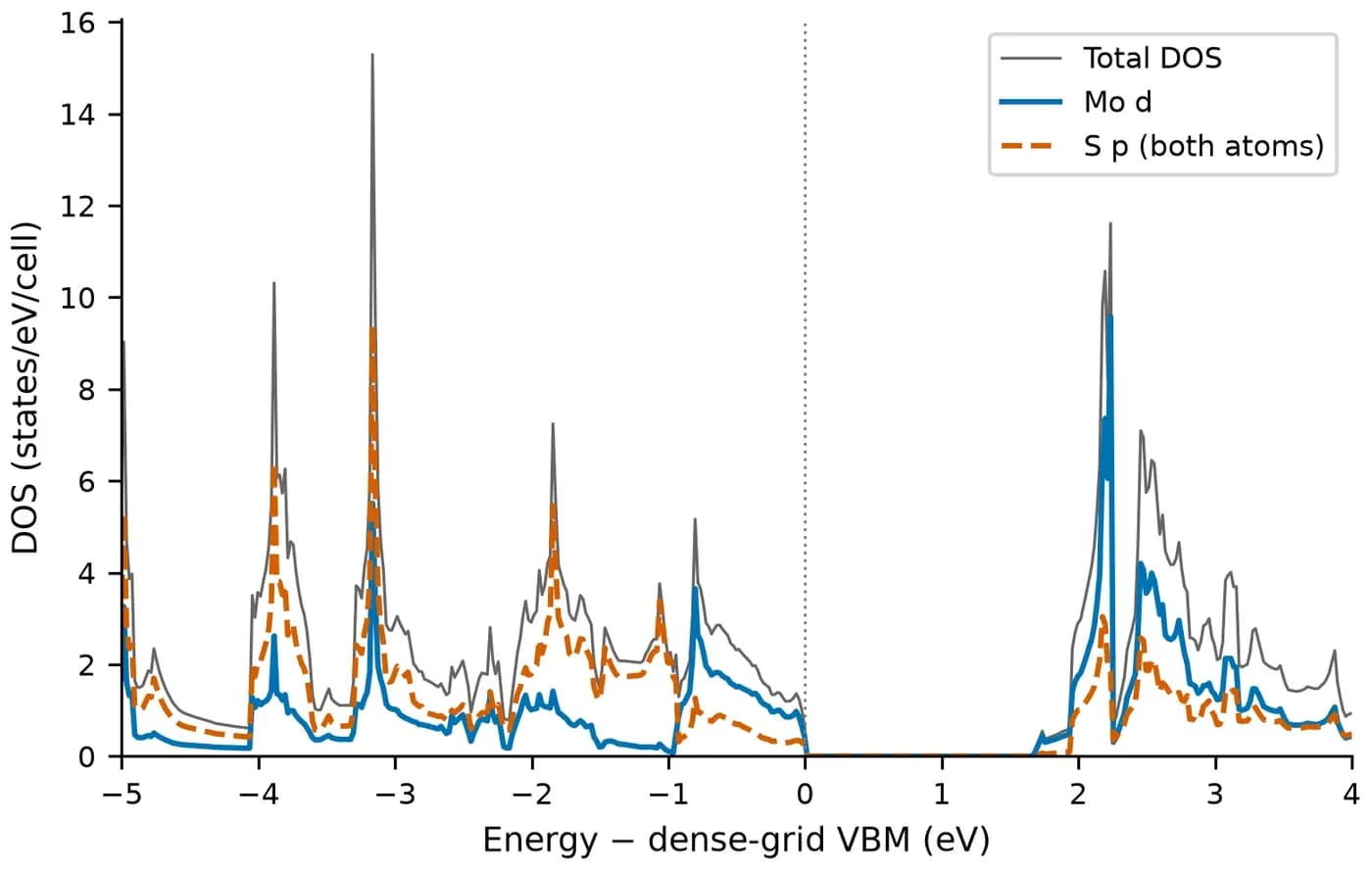
Step 7
Why this stepSOC from Mo splits the valence band at K, and this value can be compared directly with the literature.
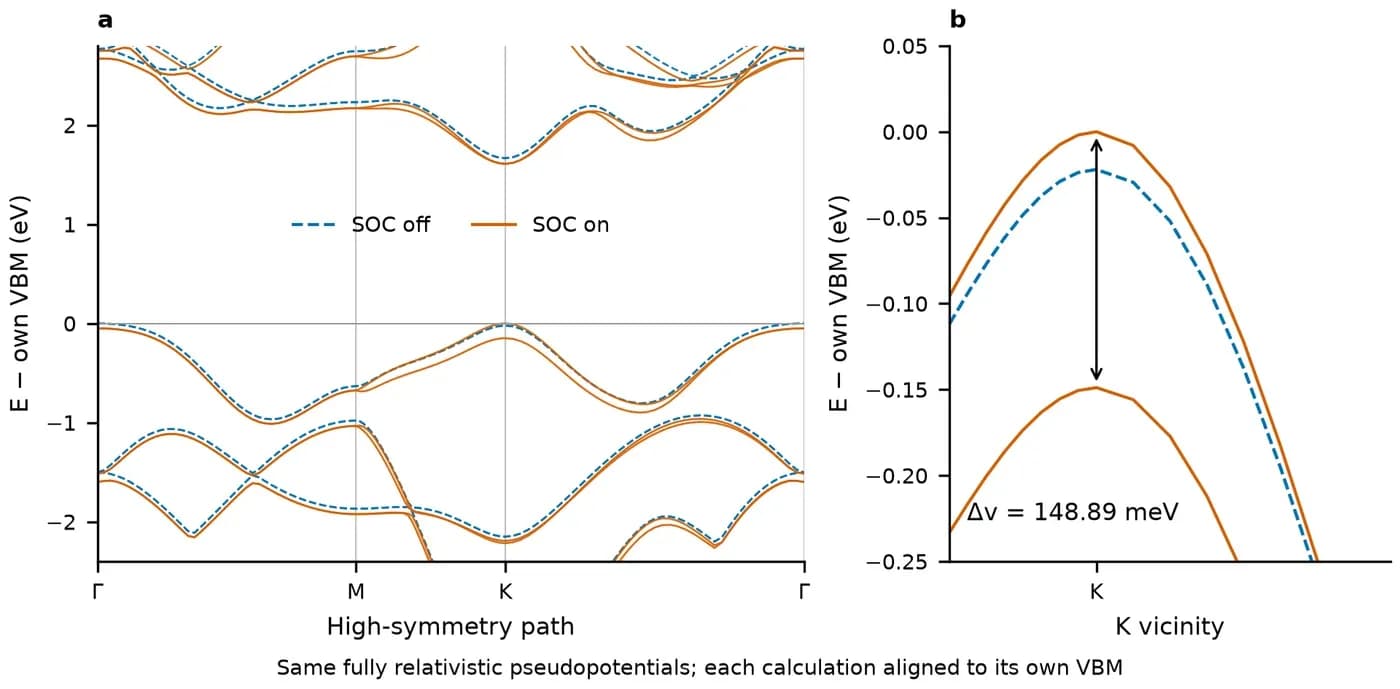
SOC needs three changes. First, use fully relativistic pseudopotentials; this guide uses SG15 Mo_ONCV_PBE_FR-1.0 and S_ONCV_PBE_FR-1.1. Second, set noncolin=.true. and lspinorb=.true. in &SYSTEM. Third, set nbnd to 36. Each band now holds one electron, so occupied bands go from 13 to 26, and the second argument of the gap script becomes 26. nspin=2 is a collinear spin calculation and cannot replace SOC.
Fully relativistic pseudopotentials need their own cutoff test, so 55 Ry cannot be reused. This guide tests up to 95 Ry and adopts 95/380 Ry.
To measure the effect of SOC, use the same fully relativistic pseudopotentials and the same structure for both runs, and switch only lspinorb. Subtracting a scalar-relativistic result from a fully relativistic one would mix in the pseudopotential difference. The structure here is fixed at the scalar-relativistic optimum. Its residual force with the fully relativistic pseudopotentials is about 0.0012 Ry/bohr, and it was not reoptimized.
The splitting at K is the energy difference between bands 26 and 25 at K: 148.89 meV. Xiao et al. (2012) give 2λ = 0.15 eV, a difference of 1.11 meV.
&SYSTEM
 ecutwfc=95, ecutrho=380, nbnd=36,
 noncolin=.true., lspinorb=.true.,
/
&ELECTRONS
 conv_thr=1d-10, mixing_beta=0.3, mixing_ndim=4, electron_maxstep=150,
/
ATOMIC_SPECIES
Mo 95.95 Mo_ONCV_PBE_FR-1.0.upf
S 32.06 S_ONCV_PBE_FR-1.1.upf| Quantity | SOC off (eV) | SOC on (eV) | Change (meV) |
|---|---|---|---|
| Fundamental gap | 1.66644 (Γ→K) | 1.60847 (K→K) | −57.98 |
| Direct gap at K | 1.68840 | 1.60847 | −79.94 |
| Valence splitting at K | 0 | 0.14889 | 148.89 |
Choose by your situation
Bulk
Why this stepLayers in bulk MoS2 are held by van der Waals forces, which PBE alone describes poorly, so they need separate treatment.
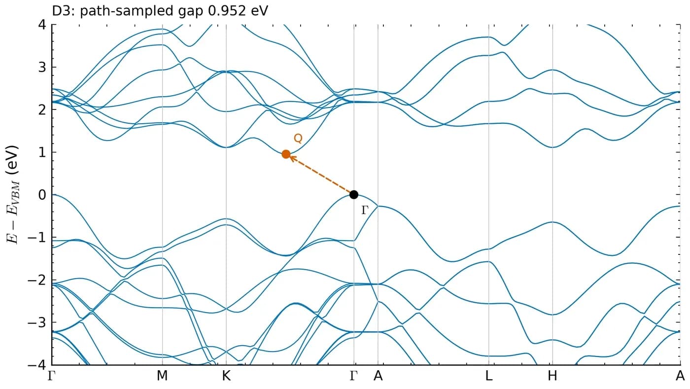
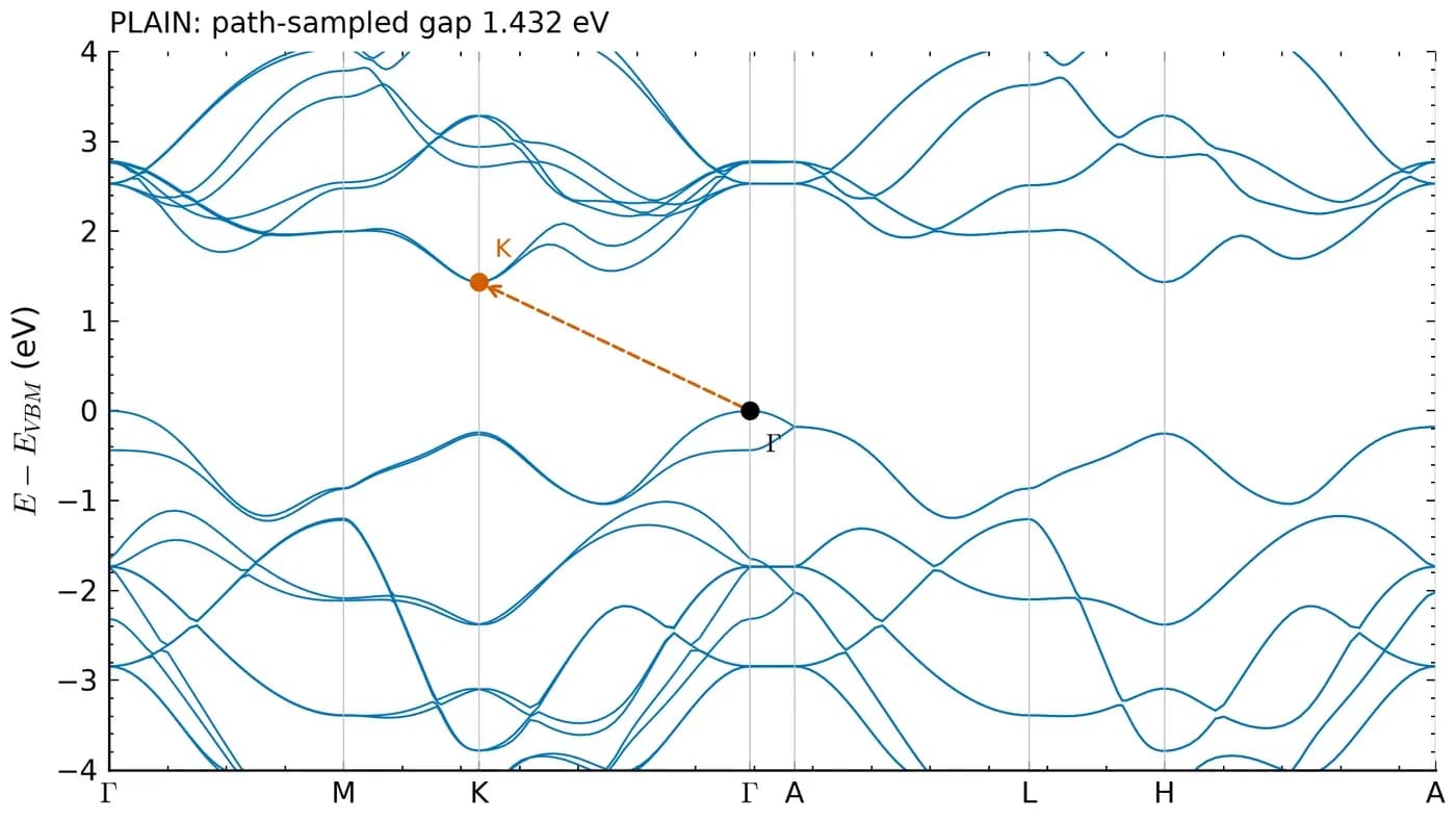
Without dispersion correction, the optimized c is 14.58 Å, 1.89 Å above the published 12.70 Å. With DFT-D3, c is 12.49 Å and the fundamental gap goes from 1.432 eV to 0.952 eV. D3 does not directly change the eigenvalues of a fixed structure, so this gap change comes mainly from the layer spacing.
The band edge in bulk does not sit at a high-symmetry point. With D3 the conduction minimum lies in the Q valley between Γ and K. On the unoptimized structure, the 12×12×4 scf mesh missed this valley and gave a gap 11.36 meV larger than path sampling, so the valley was refined locally later. Converging the scf mesh and locating the true band edge are two separate problems.
| Quantity | PBE | PBE-D3 | Kuc et al. (2011) |
|---|---|---|---|
| a (Å) | 3.1844 | 3.1673 | 3.173 |
| c (Å) | 14.5825 | 12.4894 | 12.696 |
| Fundamental gap (eV) | 1.432 (Γ→K) | 0.952 (Γ→Q) | 1.2 |
| Direct gap at K (eV) | 1.671 | 1.673 | 1.8 |
Concepts and judgment
Explanation
Why this stepMany sources describe monolayer MoS2 as direct at K. The result here without SOC differs and needs an explanation.
The valence energies at Γ and K are very close. In the scalar PBE result Γ lies 16.76 meV above K. With a difference this small, the ordering can depend on the pseudopotential and the structure, so a second pseudopotential set is needed as a check.
The fully relativistic pseudopotentials, with SOC off and on the same structure, also put Γ above K, by 21.96 meV. Both sets therefore give the same ordering for this structure and functional.
With SOC on, the valence band at K splits and its upper branch rises above Γ. The bands.x output places it about 50 meV above Γ, so the fundamental gap becomes direct at K. These results apply to the PBE functional and structure used here and cannot alone determine the gap type of the real material.
Explanation
Why this stepBefore comparing with an experimental value, confirm that both sides refer to the same kind of gap.
The PBE gap is a difference between Kohn–Sham eigenvalues. The quasiparticle gap is the energy difference between adding and removing an electron, which is what GW calculates. The optical gap is the energy of absorption or emission, and it includes the attraction between electron and hole, known as the excitonic effect.
The 1.90 eV of Mak et al. (2010) is the photoluminescence peak of monolayer MoS2, which is an optical gap. The 1.608 eV here is a PBE gap. The definitions differ, so subtracting them does not give an error. No GW or BSE was run here, so this difference is not decomposed.
| Gap | Meaning | Method |
|---|---|---|
| Kohn–Sham gap | Difference of DFT eigenvalues | PBE, used here |
| Quasiparticle gap | Energy difference of adding and removing an electron | GW, photoemission with inverse photoemission |
| Optical gap | Optical excitation energy including excitons | BSE, absorption, photoluminescence |
Reference and appendix
Comparison
Why this stepThe parameters were fixed before the literature was read, and published values were not used for tuning.
Conditions differ from this guide: Kuc et al. (2011) use a different basis and cut their monolayer from the optimized bulk. The differences below therefore cannot all be treated as errors. The bulk D3 fundamental gap is 0.25 eV below Kuc et al., and this run did not attribute that difference to a single cause.
| Quantity | This guide | Literature | Difference | Source |
|---|---|---|---|---|
| Monolayer valence splitting at K | 148.89 meV | 150 meV | −1.11 meV | Xiao 2012 |
| Monolayer a | 3.1838 Å | 3.193 Å | −0.0092 Å | Xiao 2012 |
| Monolayer direct gap at K | 1.6856 eV | 1.9 eV | −0.214 eV | Kuc 2011 |
| Bulk D3 a | 3.1673 Å | 3.173 Å | −0.0057 Å | Kuc 2011 |
| Bulk D3 c | 12.4894 Å | 12.696 Å | −0.2066 Å | Kuc 2011 |
| Bulk D3 fundamental gap | 0.9517 eV | 1.2 eV | −0.248 eV | Kuc 2011 |
| Monolayer photoluminescence peak | Not comparable | 1.90 eV | Different definition | Mak 2010 |
Run record
Why this stepThe calculation conditions, run time and checks.
This was one long-running research task on Scientify on 5 November 2026. After the brief was uploaded, the Agent chose the pseudopotentials, ran the convergence tests, optimized the structures, calculated bands and SOC, read the literature and wrote the report. It took 6 h 18 min and 354 operations, with no human intervention and no rented compute.
The calculation used only the 2-core CPU of the cloud computer, running QE 7.5 serially with one process and one thread. SOC took the longest, about 2.35 hours across 22 QE runs. The 6 h 18 min covers all convergence tests, bulk, literature and report writing. Rerunning the package from this page on the same cloud computer takes about 10 minutes for the monolayer from optimization to projected DOS, and the optimized cell matches the original run.
A separate review task run by the Agent performed the final check. It recomputed the gaps from raw XML and re-parsed the reproduction package in a new directory, and it passed. Known limits are stated in the report: the structure was not reoptimized with SOC; one k12 XML in the scalar pseudopotential sensitivity check was not kept, so that difference only has a conservative bound of about 0.29 meV; and the erratum to Qiu et al. (2013) could not be verified, so that paper is not used as a benchmark.
| Calculation | Wall time (s) | Peak memory (MiB) |
|---|---|---|
| Monolayer final scf | 56.75 | 574 |
| Monolayer optimization | 284.99 | 582 |
| Monolayer path bands | 126.39 | 510 |
| Monolayer DOS / PDOS | 5.81 / 5.92 | 485 |
| Bulk D3 optimization | 581.98 | 709 |
| Bulk D3 path bands | 375.09 | 433 |
| All 22 SOC QE runs | 8475.67 | 255 |

Troubleshooting
A restart fails with a wrong electron count or charge, for example about 0.05 instead of 52
Cause: The charge file left by an interrupted run is unusable. This happened in a bulk restart here.
Fix: Do not reuse that charge. Start from scratch. For long optimizations, stop safely in segments with max_seconds and keep the output of each segment.
The plot looks direct at K but the script reports an indirect gap
Cause: The valence energies at Γ and K differ by only tens of meV, which a plot does not show. A wrong number of occupied bands also gives a wrong result.
Fix: Check the occupied bands first: electrons divided by 2 without SOC, and the electron count with SOC. Then read the two k-points the script prints.
The gap does not change with a parameter, or changes by exactly 0.001 eV
Cause: bands.x keeps three decimals, so small differences are rounded away.
Fix: For differences below 1 meV, read eigenvalues from the XML in outdir.
The valley at K is missing, or the bands look different from published plots
Cause: The fractional coordinates of K depend on the lattice convention. They are (1/3, 1/3, 0) for the 120° vectors here and differ for other vectors.
Fix: Check the high-symmetry coordinates against your CELL_PARAMETERS before running bands.
lspinorb=.true. gives a pseudopotential error, or there is no splitting at K
Cause: Scalar-relativistic pseudopotentials were used, or only nspin=2 was set.
Fix: Use fully relativistic pseudopotentials, set noncolin=.true. and lspinorb=.true., and retest the cutoff.
df on the cloud computer shows the disk nearly full
Cause: The Scientify project disk grows on demand, and df shows its current size, which is smaller than the available capacity.
Fix: Run scientify-resources and read the total and free space on the Project disk line.
Going from 1 to 2 OpenMP threads does not speed up the run noticeably
Cause: Two threads showed no clear benefit on this 2-core cloud computer. This was not a strict paired comparison.
Fix: Test on the same small case before choosing a thread count, and keep concurrent jobs within the memory limit.
Sources
- Quantum ESPRESSO pw.x input description — Official definitions of calculation, cell_dofree, K_POINTS and others
- SSSP pseudopotential library — Pseudopotentials and recommended cutoffs for the scalar runs
- SG15 ONCV pseudopotentials — Fully relativistic pseudopotentials for the SOC runs
- Kuc, Zibouche & Heine (2011), Phys. Rev. B 83, 245213 — PBE structures and gaps of bulk and monolayer MoS2
- Xiao et al. (2012), Phys. Rev. Lett. 108, 196802 — Monolayer a and valence splitting 2λ = 0.15 eV at K
- Mak et al. (2010), Phys. Rev. Lett. 105, 136805 — Monolayer photoluminescence peak at 1.90 eV