 Scientify
About this page
How-to guide- What this page solves
- You need a grid independence study for a paper or report but are unsure how many meshes to run, which quantities to track, how small a change counts as converged, and what besides the mesh needs checking.
- Who it is for
- Graduate students and engineers running CFD or finite element simulations. You should be comfortable with relative error; OpenFOAM experience is not required.
- What you will have
- You will be able to design a defensible verification plan, know which numbers to report, and recognise when you cannot claim convergence.
- Covers
- Designing the refinement ratio across three meshes
- Choosing judging quantities, and how differently they converge
- Where the 5–10% threshold comes from and why it is weak
- Where Richardson extrapolation and GCI fit in
- Separate checks for time step and domain size, with measured effects
- How to read differences against published benchmarks
- Does not cover
- Installing and learning OpenFOAM (see the official documentation)
- Turbulence model selection (this case is laminar)
- Click-by-click steps in Fluent or COMSOL
Main steps
Step 1
Why this stepRefinement has to be systematic, or differences between meshes mean nothing.
Use at least three meshes. Two only tell you how much the answer moved; three tell you whether it is settling toward a value. A common choice is doubling the cell count at each level, or shrinking cell size by a fixed ratio in every direction.
Refine everywhere at once. Refining the far field while leaving the near-wall layer alone, or the reverse, makes adjacent results incomparable. Boundary-layer cells must be refined along with the rest.
Everything other than the mesh stays fixed: boundary conditions, discretization schemes, time step, domain size, averaging window, convergence criteria. Change any of them and the difference can no longer be attributed to the mesh.
This case uses a structured mesh around the cylinder with 4,480, 8,960 and 17,920 two-dimensional cells: 112/160/224 circumferential by 40/56/80 radial, with a total radial expansion ratio of 100 in all three. Both directions are refined together and the cell count doubles exactly at each level.
| Mesh | 2D cells | Circumferential | Radial |
|---|---|---|---|
| Coarse | 4,480 | 112 | 40 |
| Medium | 8,960 | 160 | 56 |
| Fine | 17,920 | 224 | 80 |
Step 2
Why this stepA single quantity easily gives an over-optimistic answer.
Pick quantities that represent your research goal and that are sensitive to resolution. Reporting one integral quantity such as mean drag usually overstates convergence, because integral quantities converge faster than local or fluctuating ones.
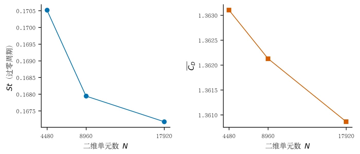
This case tracks three: the Strouhal number St (dimensionless shedding frequency), the mean drag coefficient Cd, and the lift coefficient RMS Cl,rms. The measured adjacent changes below differ sharply between them.
Mean drag barely moves from coarse to fine (0.07%, 0.09%). Judging by that alone, the coarse mesh would look sufficient. On the same meshes, lift RMS moves 3.85% from coarse to medium and only drops to 0.33% at medium-to-fine. Fluctuating quantities converge more slowly than means; this is general, not specific to this case.
State how each quantity is averaged. Here statistics are taken only after the flow reaches a stable periodic state, with cycles delimited by the upward zero crossings of lift and integrated over whole cycles. An earlier attempt used peak times, but small ripples near the peak disturbed peak location, so zero crossings were used instead.
| Comparison | St | Mean Cd | Cl,rms |
|---|---|---|---|
| Coarse → medium | −1.51% | −0.07% | +3.85% |
| Medium → fine | −0.46% | −0.09% | +0.33% |
Concepts and judgment
Criteria
Why this stepWhat is wrong with the most repeated rule, and what to use instead.
Most tutorials state that a difference under 5–10% between adjacent meshes means grid independence. The number has no agreed source, and what counts as reasonable varies widely by field and by quantity. Treating it as a universal pass mark has two problems: 5% is very loose for an integral quantity, and the rule only describes how much adjacent meshes differ, not how far you are from the true value.
A small adjacent change does not mean a small error. Under continued refinement each step shrinks by construction, so taking the last step as the total error systematically underestimates it. The rigorous approach is Richardson extrapolation: use three systematically refined meshes to estimate the observed order of convergence and an extrapolated value, then compute the grid convergence index (GCI), which carries a safety factor. Report GCI rather than adjacent change when you need a numerical uncertainty.
This page reports adjacent change and says so explicitly; the 0.33% medium-to-fine figure is not presented as an error bound. A paper that requires numerical uncertainty would need Richardson extrapolation on the same data.
A more practical rule: decide how much precision your conclusion needs. If the conclusion is that design A has 2% less drag than design B, a 5% mesh error makes it meaningless. If you are only comparing flow regimes qualitatively, the bar is lower. Derive the threshold from the precision your conclusion needs, not from a generic number.
Main steps
Step 3
Why this stepThe mesh is one of three discretization parameters; checking it alone is over-optimistic.
In unsteady problems the time step is as much a discretization parameter as the mesh, and the domain size sets how much the boundaries disturb the flow. Check both on the final mesh, changing one at a time and nothing else.
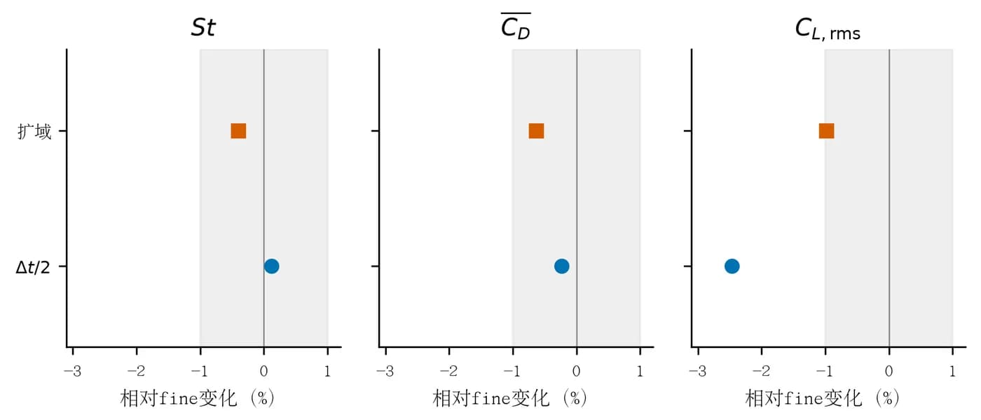
This case ran two such comparisons on the fine mesh. Halving the time step from 0.01 to 0.005 barely moved the Strouhal number or the drag, but lift RMS changed by 2.47%, far more than the 0.33% from the mesh. Enlarging the domain from [-15, 25] × [-15, 15] to [-20, 35] × [-20, 20] moved all three quantities by 0.4% to 1.0%.
So with these settings the mesh check passes and the time-step check does not. By this case's own criterion, the lift result cannot be called discretization independent: either keep reducing the time step until the change falls within the threshold, or state the limitation explicitly.
This is the risk of checking only the mesh. Seeing all three quantities under 1% from medium to fine, it is tempting to write that grid independence was verified and the results are reliable. The real limit here is the time step.
| Comparison | St | Mean Cd | Cl,rms |
|---|---|---|---|
| Mesh: medium → fine | −0.46% | −0.09% | +0.33% |
| Time step: 0.01 → 0.005 | +0.12% | −0.23% | −2.47% |
| Domain: enlarged | −0.41% | −0.63% | −0.98% |
Step 4
Why this stepGet the window wrong and every comparison above becomes incomparable.
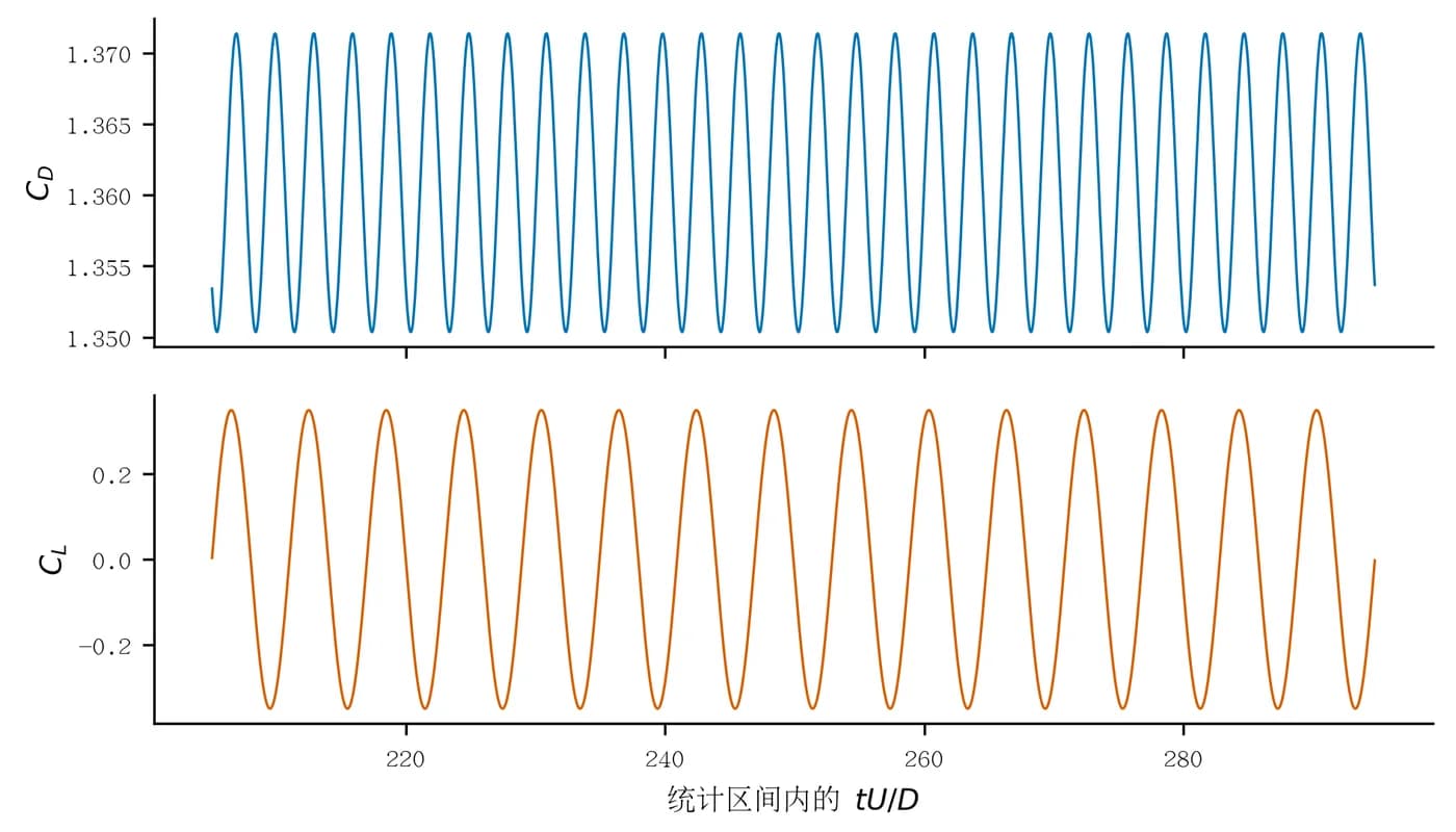
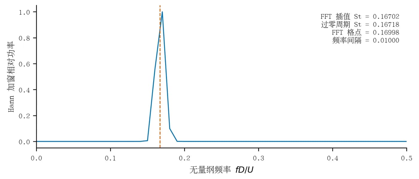
For periodic flow, wait for the initial transient to pass and shedding to stabilise before averaging. "The curve looks periodic" is not a criterion; give checkable numbers: drift of the statistics from cycle to cycle, the standard deviation of cycle length, and agreement between two independent frequency estimates.
Here the approach was to take whole cycles inside the stable window and compare the mean over the first half against the second half. On the fine mesh the cycle-to-cycle drift stays below 0.021%, and the FFT and peak-to-peak frequency estimates differ by about 0.024%. Both are small, so the window holds.
Every mesh and every comparison must use the same averaging rule. The time-step comparison here restarts from the fine-mesh field at t = 300, runs to 420, discards 300–320 as transition and averages 320–420; the baseline averages 200–300. The restart field was verified byte-for-byte identical.
Concepts and judgment
Comparison
Why this stepMatching the literature is not evidence of convergence.
Agreement with published results is often treated as proof that verification passed. The problem is that for the same standard case, published values themselves scatter considerably, because domains, resolutions, methods and averaging all differ.
This case compares against four public benchmarks. Mean drag runs from 1.319 to 1.501, a spread of 14%; Strouhal number from 0.1648 to 0.172. The present result, Cd = 1.36086 and St = 0.16718, falls inside that range, very close to one source and 9% from another. Landing inside the published range is a low bar and does not constitute verification.
Check which quantity each paper actually reports. Lift is sometimes given as RMS and sometimes as half peak-to-peak amplitude, and the two differ by a factor of √2. Here Cl,rms = 0.24669 and half peak-to-peak = 0.34909, a ratio of 1.415. Comparing your RMS against someone else's amplitude invents a 41% discrepancy.
Use the literature as an order-of-magnitude check: a result far outside the published range means something is wrong with the setup. Landing inside it only means there is no obvious error; convergence still has to be demonstrated by your own comparisons.
| Source | St | Deviation | Mean Cd | Deviation |
|---|---|---|---|---|
| Qu et al. (2013) | 0.1648 | +1.44% | 1.319 | +3.17% |
| Layton et al. (2016) | 0.166 | +0.71% | 1.37 | −0.67% |
| Uhlmann (2005), enlarged domain | 0.169 | −1.08% | 1.453 | −6.34% |
| Uhlmann (2005), original domain | 0.172 | −2.80% | 1.501 | −9.34% |
Reference and appendix
Case setup
Why this stepA setup you can rerun and compare against your own case.
The solver is pisoFoam (incompressible, unsteady, laminar). Force coefficients come from OpenFOAM's own forceCoeffs function object; for a two-dimensional case note that the reference area is the diameter times the spanwise thickness.
Key settings for the fine-mesh case are below. The complete 0, constant and system directories are downloadable; unpack them and run blockMesh followed by pisoFoam.
application     pisoFoam;
endTime         312;
deltaT          0.01;
writeControl    runTime;
writeInterval   0.2;

functions
{
    forces
    {
        type        forceCoeffs;
        libs        ("libforces.so");
        patches     (cylinder);
        rho         rhoInf;
        rhoInf      1;
        liftDir     (0 1 0);
        dragDir     (1 0 0);
        magUInf     1;
        lRef        1;        // cylinder diameter D
        Aref        0.1;      // D x spanwise thickness, one cell thick in 2D
        writeControl timeStep;
        writeInterval 1;
    }
}tar xzf openfoam-cylinder-case-fine.tar.gz
cd fine
blockMesh
checkMesh
pisoFoam | tee log.pisoFoam
# coefficients land in postProcessing/forces/0/coefficient.dat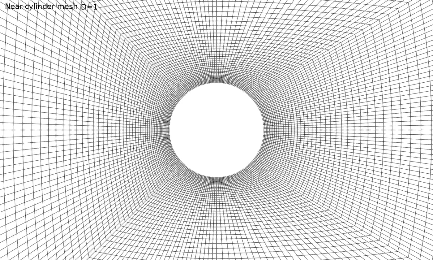
- openfoam-cylinder-case-fine.tar.gzThe 0, constant and system directories for the fine mesh (OpenFOAM v2412). Change the circumferential and radial divisions in blockMeshDict to get the coarse and medium meshes.
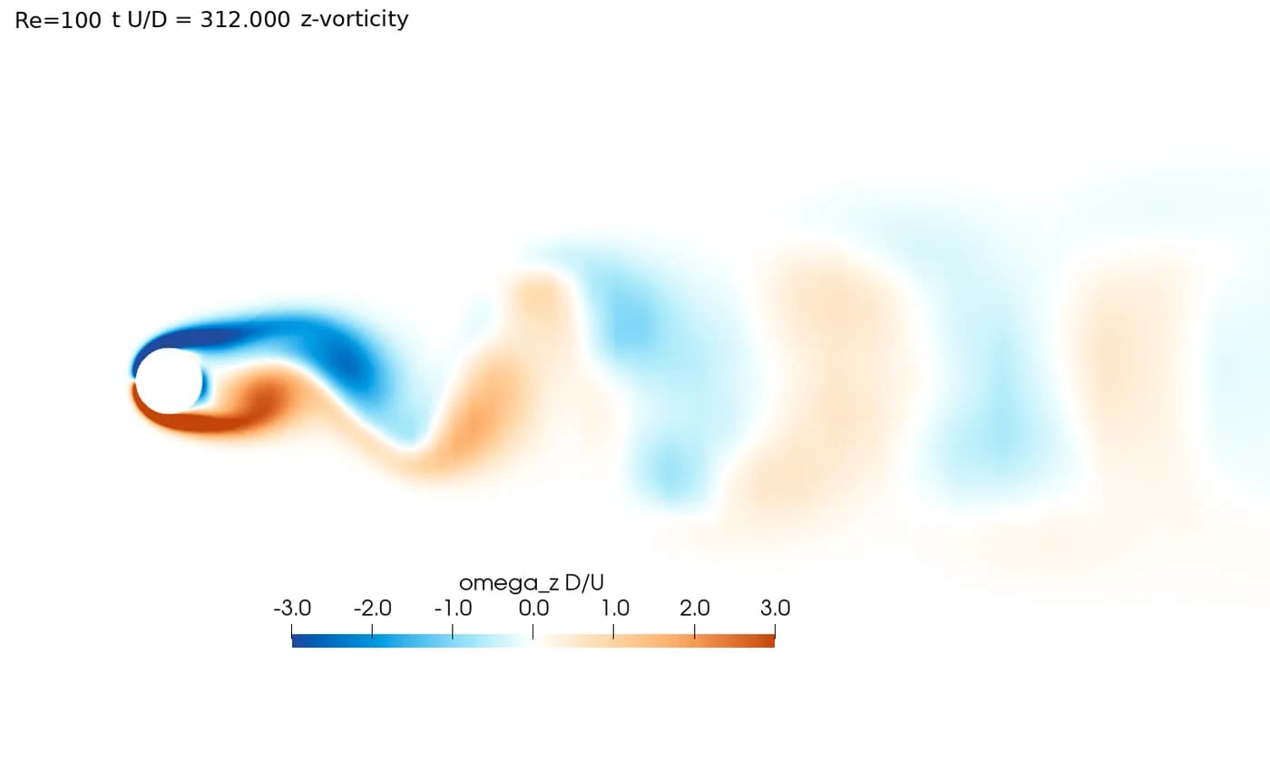
- vorticity.mp4Vorticity animation, 61 frames covering about 2.01 shedding cycles, rendered offscreen with ParaView.
Run record
Why this stepCompute conditions, effort and how the numbers were checked.
A long-running research task on Scientify on 4 November 2026. After a brief was uploaded, the platform designed the meshes, built five cases (three meshes plus the time-step and domain comparisons), ran them, computed the statistics, searched the literature and produced the figures — 1 hour 27 minutes in total, on two CPU cores of a cloud computer, with no GPU rented.
Three independent reviews followed: literature sources, numerical setup, and a final review. The final review recomputed Cd, Cl,rms, zero-crossing frequency and FFT frequency from the raw force files of all five cases and matched the delivered tables exactly; it also checked the report PDF page by page, compared the Excel sheets cell by cell, and verified 1,308 file hashes in the reproduction archive.
The vorticity animation has 61 frames corresponding to 61 saved fields between t = 300 and 312, covering about 2.01 shedding cycles. It was rendered offscreen through ParaView with no graphical display.

Troubleshooting
Results oscillate across the three meshes instead of settling
Cause: You are not yet in the convergent range, refinement was not systematic (some regions were not refined), or the averaging window is too short.
Fix: Confirm the refinement ratio is consistent in every direction and that boundary-layer cells were refined too; then extend the averaging time. If it still oscillates, add a finer mesh and see whether the trend becomes monotonic.
Mean quantities stopped changing long ago, yet a reviewer still questions the resolution
Cause: Only integral quantities were used. They converge much faster than local or fluctuating ones.
Fix: Add a fluctuating or local quantity, such as lift RMS here. In this case mean drag moved 0.09% while lift RMS was still moving 0.33%.
The mesh check passes but results still disagree with the literature
Cause: The time step or the domain was never checked. In unsteady problems the time step is often the real bottleneck.
Fix: On the final mesh, halve the time step and rerun, then enlarge the domain and rerun, and record each change. Here the time step mattered about seven times more than the mesh.
Lift differs from the literature by roughly 40%
Cause: RMS is being compared against half peak-to-peak amplitude. For a near-sinusoidal signal they differ by √2, about 41%.
Fix: Check which one the source reports. Here Cl,rms = 0.24669 and half peak-to-peak = 0.34909, a ratio of 1.415.
The same mesh gives different answers for different averaging windows
Cause: The window falls inside the initial transient or a transition segment, or does not cover whole cycles.
Fix: Average over whole cycles and report the first-half versus second-half drift plus the standard deviation of cycle length. Here the drift stays below 0.021%.
Sources
- Qu et al. (2013), Re=100 cylinder benchmark — St 0.1648, Cd 1.319, Cl,rms 0.2253
- Layton, Krishnan & Barba (2016), cuIBM — St 0.166, Cd 1.37±0.009, Cl ±0.339
- Uhlmann (2005) immersed boundary, values via arXiv:1809.08170 — Original and enlarged domain results
- OpenFOAM User Guide