 Scientify
About this page
Tutorial- What this page solves
- Your policy reached different regions in different years, and a reviewer asked you not to report only a two-way fixed effects result. You do not know how to run a Bacon decomposition, how to use Callaway–Sant'Anna, or whether the gap to TWFE matters.
- Who it is for
- Graduate students in economics, public administration and public health who evaluate policies. You know the two-period, two-group DiD and use R or are willing to learn it.
- What you will have
- You can run TWFE, the Bacon decomposition, the Callaway–Sant'Anna overall effect and the event-study plot on your own panel, and judge whether the TWFE result can be trusted.
- Covers
- TWFE baseline and clustered standard errors
- Goodman-Bacon decomposition and the weights of the three 2×2 comparison types
- Callaway–Sant'Anna ATT(g,t), overall effects and event study
- Cross-checks with Sun–Abraham and imputation estimators
- Parallel-trends tests, HonestDiD sensitivity analysis and a permutation test
- Comparison with the papers and official documentation
- Does not cover
- Line-by-line Stata usage (only the mapping to R packages)
- Synthetic control and synthetic DiD
- Triple differences
- DiD with continuous treatment intensity
Main steps
Step 1
Why this stepThe input of a staggered DiD is a panel with one row per unit and period, plus each unit's first treatment year. Start by checking the timing and the size of each cohort.
The minimum wage data is mpdta, shipped with the R package did: 500 counties, 2003–2007, and the log of teen employment (lemp) as the outcome. Counties first raised the minimum wage in 2004, 2006 or 2007, and 309 counties never did within the sample. The did documentation says it is a subset of the data in the Callaway and Sant'Anna paper.
The castle doctrine data is the state panel used by Cheng and Hoekstra (2013): 50 states, 2000–2010, and the log homicide rate (l_homicide) as the outcome. 29 states were never treated, and the other 21 states took effect in five cohorts between 2005 and 2009. The data come from Cunningham's Mixtape repository.
In the did package the first treatment year is called gname, and never-treated units are coded 0. The treatment status D equals 1 from the first treatment year on.
library(did); library(fixest); library(bacondecomp)
data(mpdta, package = "did")
d <- mpdta
d$D <- as.integer(d$first.treat > 0 & d$year >= d$first.treat)
table(unique(d[c("countyreal", "first.treat")])$first.treat)| Data | First treatment year and number of units | Never treated | Total |
|---|---|---|---|
| Minimum wage (counties) | 2004:20;2006:40;2007:131 | 309 | 500 |
| Castle doctrine (states) | 2005:1;2006:13;2007:4;2008:2;2009:1 | 29 | 50 |
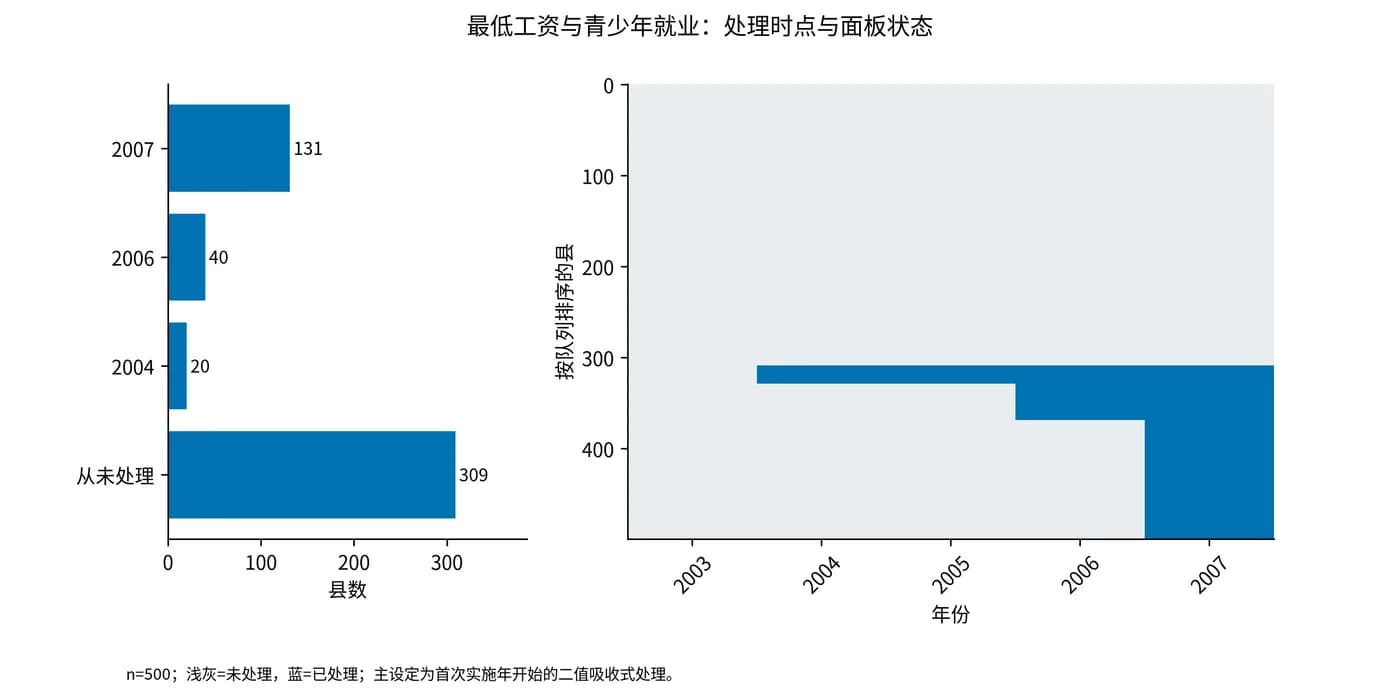
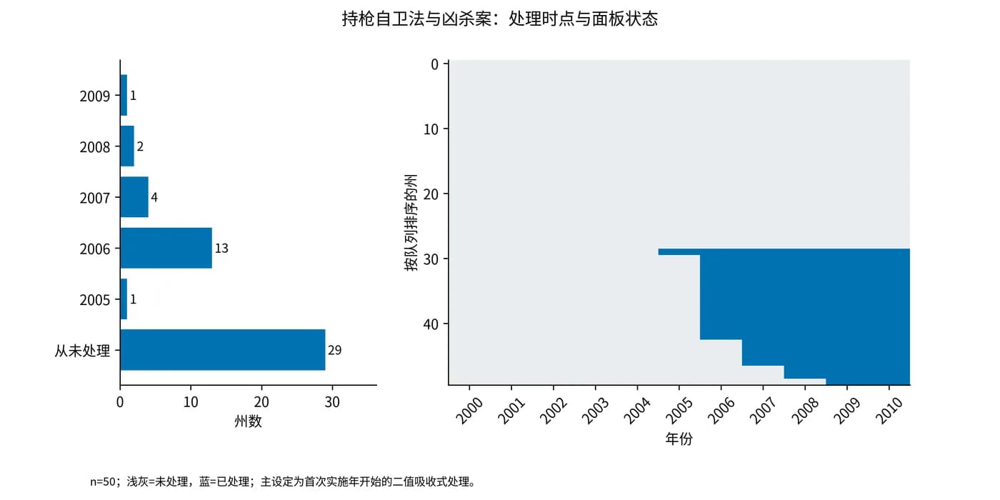
Step 2
Why this stepTWFE regresses the treatment status D on unit and time fixed effects. Reviewers expect it, and every later estimator is compared with it.
Standard errors are clustered by unit: counties in mpdta and states in the castle data. On the minimum wage data the TWFE coefficient is -0.0365 with a standard error of 0.0133. On the castle data it is 0.0818 with a standard error of 0.0589 and a 95% confidence interval of [-0.037, 0.200].
The outcome is in logs, so a coefficient is roughly a percentage change: -0.0365 is about a 3.6% fall in teen employment, and 0.0818 is about an 8.5% rise in the homicide rate.
twfe <- feols(lemp ~ D | countyreal + year, d, cluster = ~countyreal)
coeftable(twfe)Step 3
Why this stepThe TWFE estimate is a weighted average of all 2×2 DiD comparisons. The Goodman-Bacon decomposition lists each comparison and its weight, so you can see what TWFE relies on.
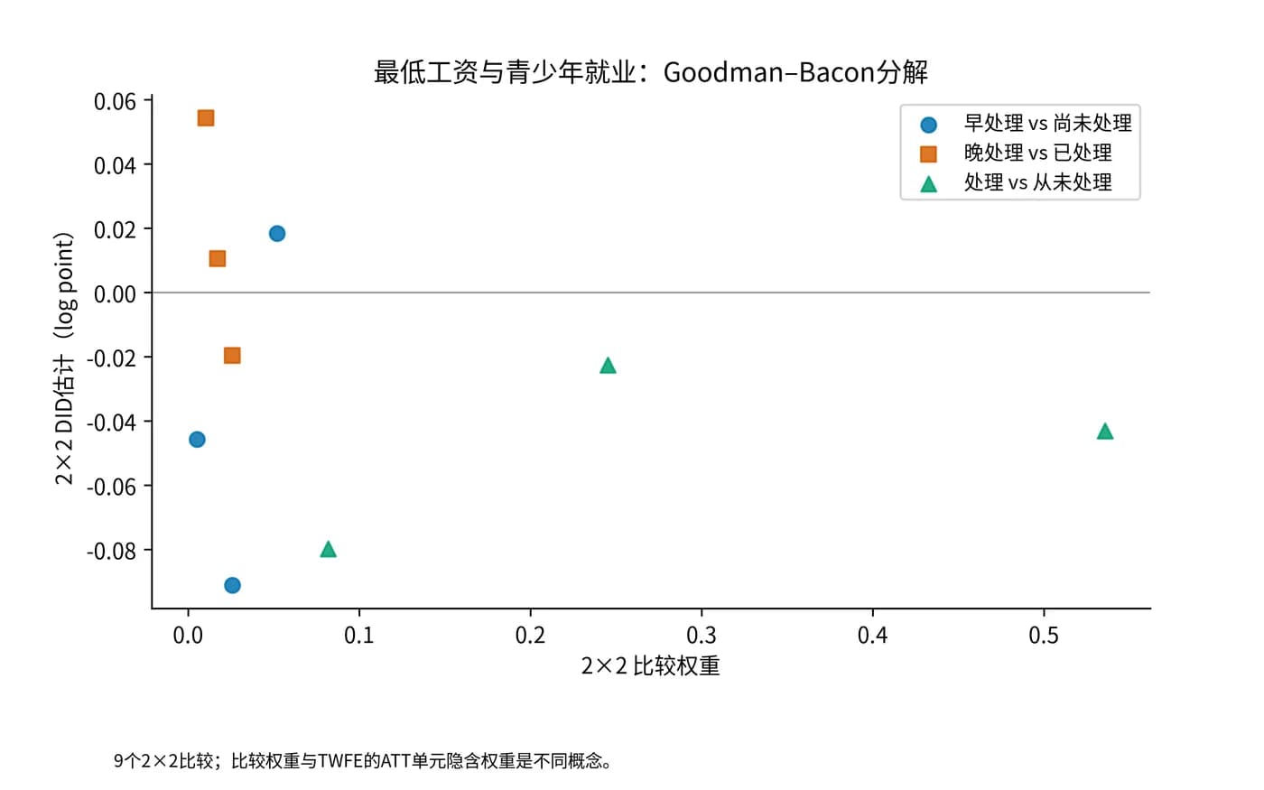
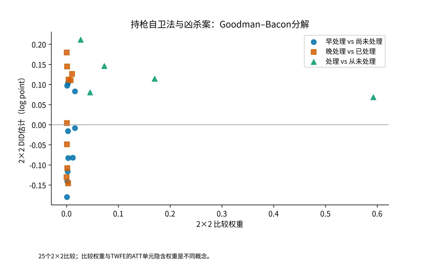
The comparisons fall into three types. Treated versus never treated. Earlier-treated versus later-treated, where the later group serves as the control before it is treated. And later-treated versus earlier-treated, where the already-treated earlier group serves as the control. In the third type the control group's own treatment effect enters the estimate, which biases it when effects change over time.
In both datasets the treated-versus-never-treated comparisons carry most of the weight, 86.3% and 90.8%. Comparisons that use an already-treated group as the control carry less, 5.4% and 3.2%. The three weights add to one, and TWFE equals the sum of weight times estimate over the comparisons. In this run the identity holds with an error below 10⁻¹⁰.
b <- bacon(lemp ~ D, data = d, id_var = "countyreal", time_var = "year", quietly = TRUE)
types <- do.call(rbind, lapply(split(b, b$type), function(x)
  data.frame(type = x$type[1], weight = sum(x$weight),
estimate = sum(x$weight * x$estimate) / sum(x$weight))))| Comparison type | mpdta weight | mpdta mean estimate | Castle weight | Castle mean estimate |
|---|---|---|---|---|
| Treated vs never treated | 0.8628 | -0.0407 | 0.9083 | 0.0880 |
| Earlier vs later treated | 0.0833 | -0.0198 | 0.0598 | -0.0055 |
| Later vs earlier treated (already-treated control) | 0.0539 | 0.0046 | 0.0319 | 0.0703 |
Step 4
Why this stepThe Callaway–Sant'Anna estimator first estimates an average treatment effect ATT(g,t) for each treatment cohort g and period t, using only units that are not yet treated as controls, and then aggregates them.
Controls are never-treated units (control_group = "nevertreated"). est_method = "dr" is doubly robust, and without covariates its point estimates equal those of "reg" and "ipw". base_period = "universal" uses the period before treatment (e = -1) as the base for all comparisons, so pre-treatment coefficients in the event-study plot can be compared with zero directly. Confidence intervals use the multiplier bootstrap with 999 draws, clustered by unit.
The minimum wage data have 7 post-treatment ATT(g,t). For the 2004 cohort the four estimates are -0.0105 in 2004, -0.0704 in 2005, -0.1373 in 2006 and -0.1008 in 2007. These four numbers match the official did documentation.
set.seed(20261106)
gt <- att_gt(yname = "lemp", tname = "year", idname = "countyreal", gname = "first.treat",
             data = d, control_group = "nevertreated", est_method = "dr",
             base_period = "universal", bstrap = TRUE, biters = 999,
             clustervars = "countyreal", cband = TRUE)
summary(gt)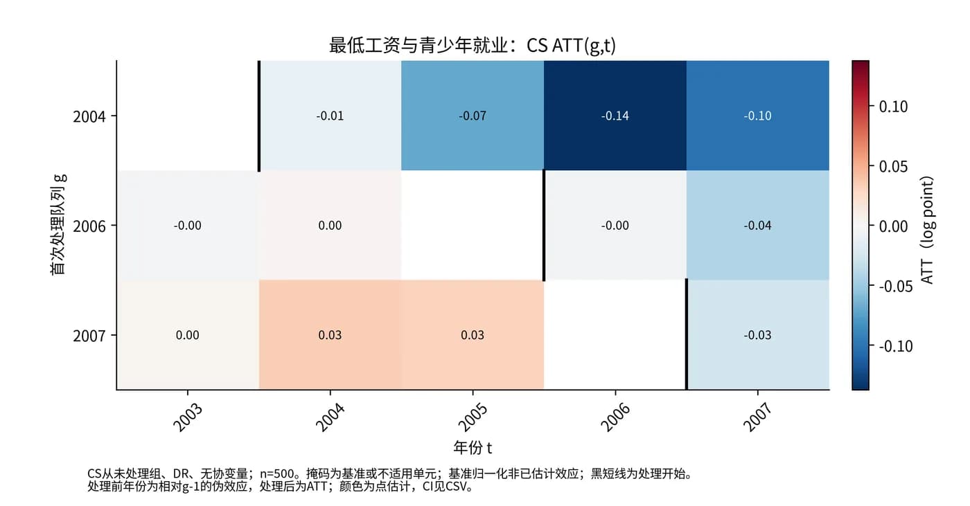
Step 5
Why this stepSeven ATT(g,t) cannot go into a paper as they are and need aggregation. aggte offers several ways to do it, and each answers a different question.
simple takes a weighted average of all post-treatment ATT(g,t) by cohort size. For mpdta it is -0.0400 with a standard error of 0.0122. dynamic aggregates by years since treatment (event time e) and then averages over event times: e = 0 to 3 give -0.0199, -0.0510, -0.1373 and -0.1008, and their mean is -0.0772 with a standard error of 0.0203. This dynamic overall effect matches the -0.0772 (standard error 0.0203) in the official did documentation.
The two overall effects answer different questions, so one cannot replace the other. Say which one you report. The event-study plot comes from the per-period results of dynamic, and e = -1 is the base period with no standard error.
set.seed(20261106); simple  <- aggte(gt, type = "simple",  bstrap = TRUE, biters = 999, clustervars = "countyreal")
set.seed(20261106); dynamic <- aggte(gt, type = "dynamic", bstrap = TRUE, biters = 999, clustervars = "countyreal")
ggdid(dynamic)   # 事件研究图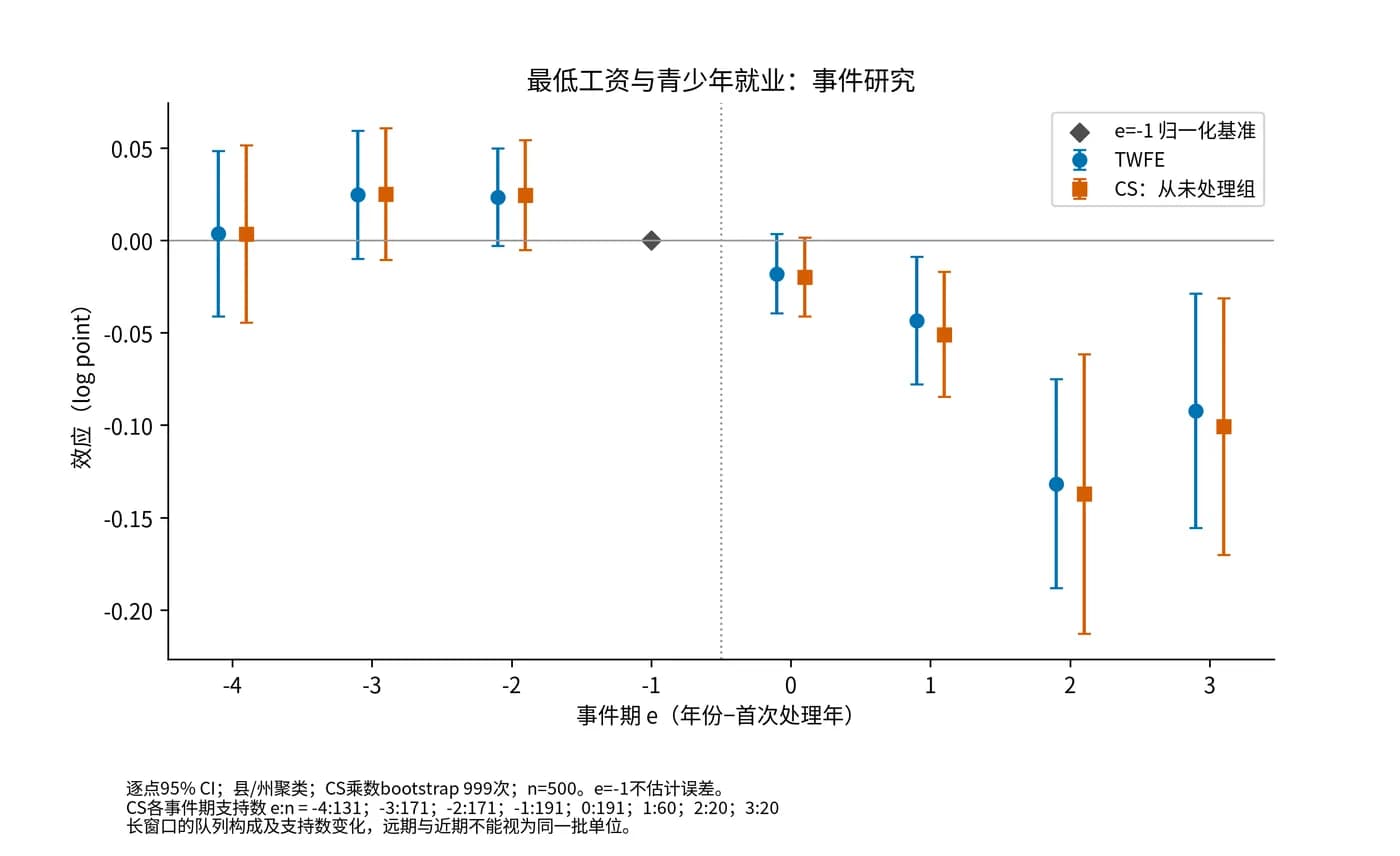
Step 6
Why this stepParallel trends means that without the policy, treated and control groups would have moved in parallel. It cannot be tested directly. You can only check whether the pre-treatment event-study coefficients are close to zero.
For mpdta the pre-treatment coefficients are 0.0033 at e = -4, 0.0250 at e = -3 and 0.0245 at e = -2, with standard errors between 0.015 and 0.024. The joint test of the three has p = 0.168, and the same test on the TWFE event study gives p = 0.181. Neither rejects.
In the castle data separate near and far leads. The coefficients at e = -6 to -2 lie between -0.008 and 0.058 with standard errors of 0.05 to 0.07. The coefficients at e = -9 to -7 are -0.404, -0.124 and -0.233, but these three periods are observed in only 1, 3 and 7 states, while the near periods have 20 to 21 states. The joint test over all pre-treatment coefficients has p below 0.001, and the test on e = -4 to -2 alone has p = 0.186. The far leads have too little data to weigh the same as the near ones.
Pre-treatment coefficients near zero do not prove parallel trends, and the test has limited power. Step 8 uses HonestDiD to answer a different question: how large a violation the conclusion can take.
gt$Wpval        # att_gt 的处理前联合检验
ggdid(dynamic)  # 处理前系数应接近 0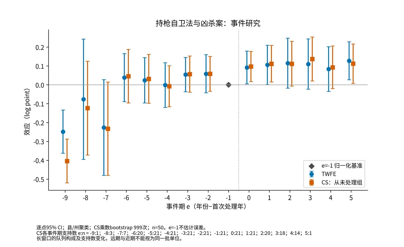
Step 7
Why this stepThe conclusion should not depend on a single estimator. Sun–Abraham and Borusyak–Jaravel–Spiess (BJS) imputation are two common alternatives. Estimate once with each on the same data.
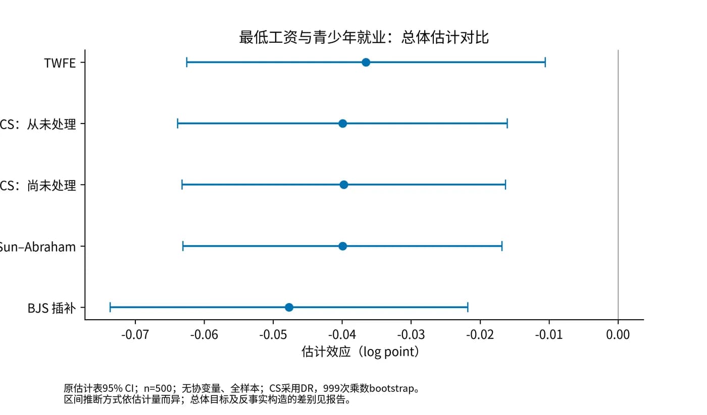
Sun–Abraham is implemented by sunab in fixest. It also uses never-treated units as controls, so its point estimate equals Callaway–Sant'Anna and only the standard error differs a little. BJS imputation fits the counterfactual on all untreated observations and compares it with treated observations, implemented in the didimputation package.
On the minimum wage data every estimator except BJS (-0.0477) lies between -0.0365 and -0.0400. On the castle data TWFE is 0.0818, Callaway–Sant'Anna and Sun–Abraham are 0.1104, and BJS is 0.0798. The differences are all smaller than the standard errors (about 0.012 for mpdta and 0.04 to 0.06 for the castle data), so a sample of this size cannot tell the estimators apart.
d$g_sa <- ifelse(d$first.treat == 0, 9999, d$first.treat)
sa  <- feols(lemp ~ sunab(g_sa, year, ref.p = -1) | countyreal + year, d, cluster = ~countyreal)
aggregate(sa, agg = "ATT")
bjs <- did_imputation(d, yname = "lemp", gname = "first.treat", tname = "year",
idname = "countyreal", first_stage = ~ 0 | countyreal + year, cluster_var = "countyreal")| Estimator | mpdta estimate (SE) | Castle estimate (SE) |
|---|---|---|
| TWFE | -0.0365 (0.0133) | 0.0818 (0.0589) |
| Callaway–Sant'Anna, never treated | -0.0400 (0.0122) | 0.1104 (0.0420) |
| Callaway–Sant'Anna, not yet treated | -0.0398 (0.0120) | 0.1094 (0.0389) |
| Sun–Abraham | -0.0400 (0.0118) | 0.1104 (0.0413) |
| BJS imputation | -0.0477 (0.0132) | 0.0798 (0.0609) |
Step 8
Why this stepHonestDiD asks how far parallel trends may be violated after treatment before the conclusion fails. A permutation test builds a reference distribution by randomly reassigning treatment timing when asymptotic theory is hard to trust.
The HonestDiD relative-magnitude restriction is written Mbar: the post-treatment trend deviation is at most Mbar times the largest pre-treatment deviation. Mbar = 0 gives the usual confidence interval. Taking the mpdta event study as input, the effect at e = 0 has the interval [-0.0429, 0.0031] at Mbar = 0, which already contains zero. The weighted average of post-treatment effects is [-0.0629, -0.0172] at Mbar = 0 and [-0.0723, -0.0068] at Mbar = 0.25, both excluding zero, and [-0.0860, 0.0073] at Mbar = 0.5, which contains zero.
So the conclusion that the average post-treatment effect is negative survives a violation of up to 0.25 times the largest pre-treatment deviation, and fails at 0.5 times. The equally weighted dynamic average in the castle data looks similar: [0.040, 0.180] at Mbar = 0 and [-0.036, 0.256] at Mbar = 0.25.
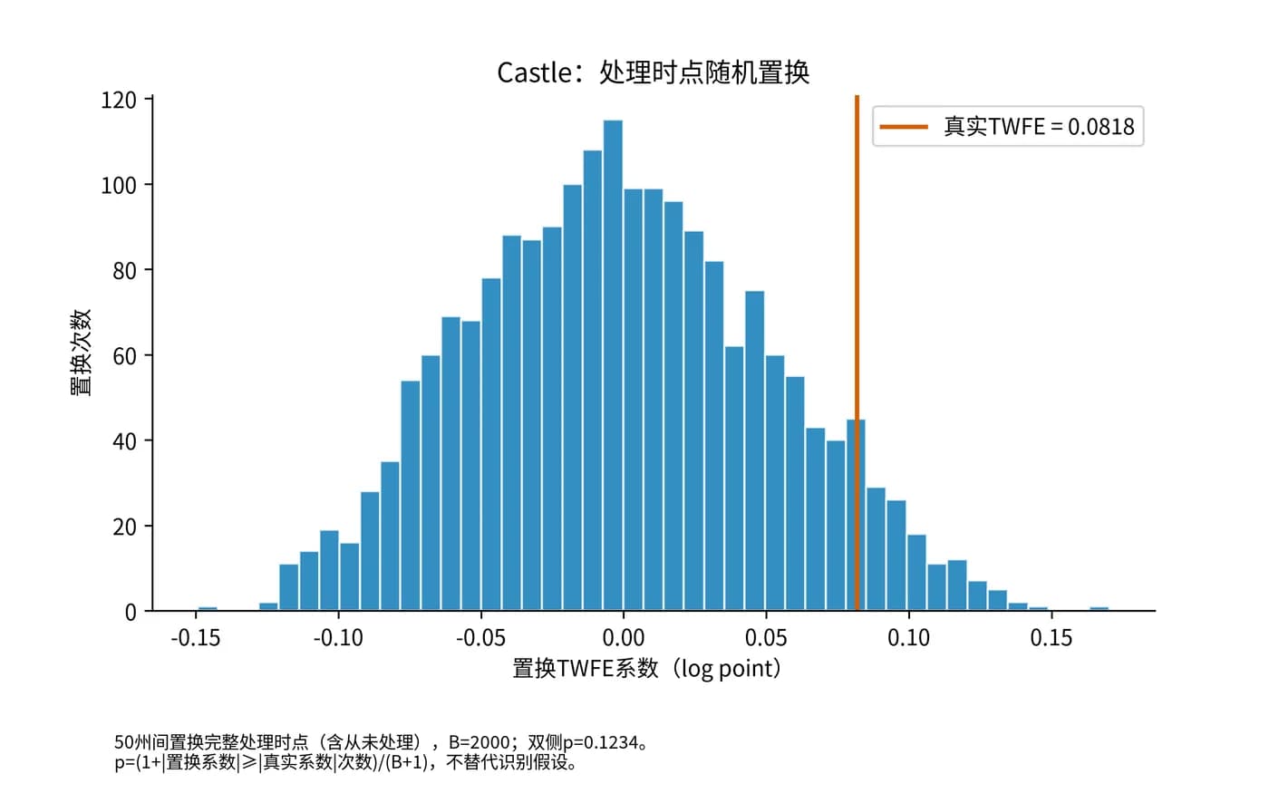
The permutation test uses the castle data. The treatment years of the 50 states are randomly reassigned across states 2000 times and the TWFE coefficient is recomputed each time. Against the permutation distribution the observed 0.0818 has 246 permutations with an absolute coefficient at least as large, so p = (1 + 246) / 2001 = 0.123. This agrees with the TWFE t-test (p = 0.171): with TWFE this dataset cannot reject a zero effect. Chinese-language papers often call this kind of random assignment and re-estimation a placebo test.
IF <- dynamic$inf.function$dynamic.inf.func.e
V  <- crossprod(IF) / nrow(IF)^2
keep <- dynamic$egt != -1
res <- createSensitivityResults_relativeMagnitudes(
  betahat = dynamic$att.egt[keep], sigma = V[keep, keep],
  numPrePeriods = 3, numPostPeriods = 4,
Mbarvec = c(0, 0.25, 0.5, 1, 2), l_vec = c(191, 60, 20, 20) / 291, alpha = 0.05)gp <- sample(g0) # g0 是各州的处理年份
Dm <- outer(gp, yrs, function(g, t) as.numeric(g > 0 & t >= g))
Dm <- Dm - rowMeans(Dm); Dm <- sweep(Dm, 2, colMeans(Dm), "-")
sum(Dm * Y) / sum(Dm^2) # 去掉两个固定效应后的 TWFE 系数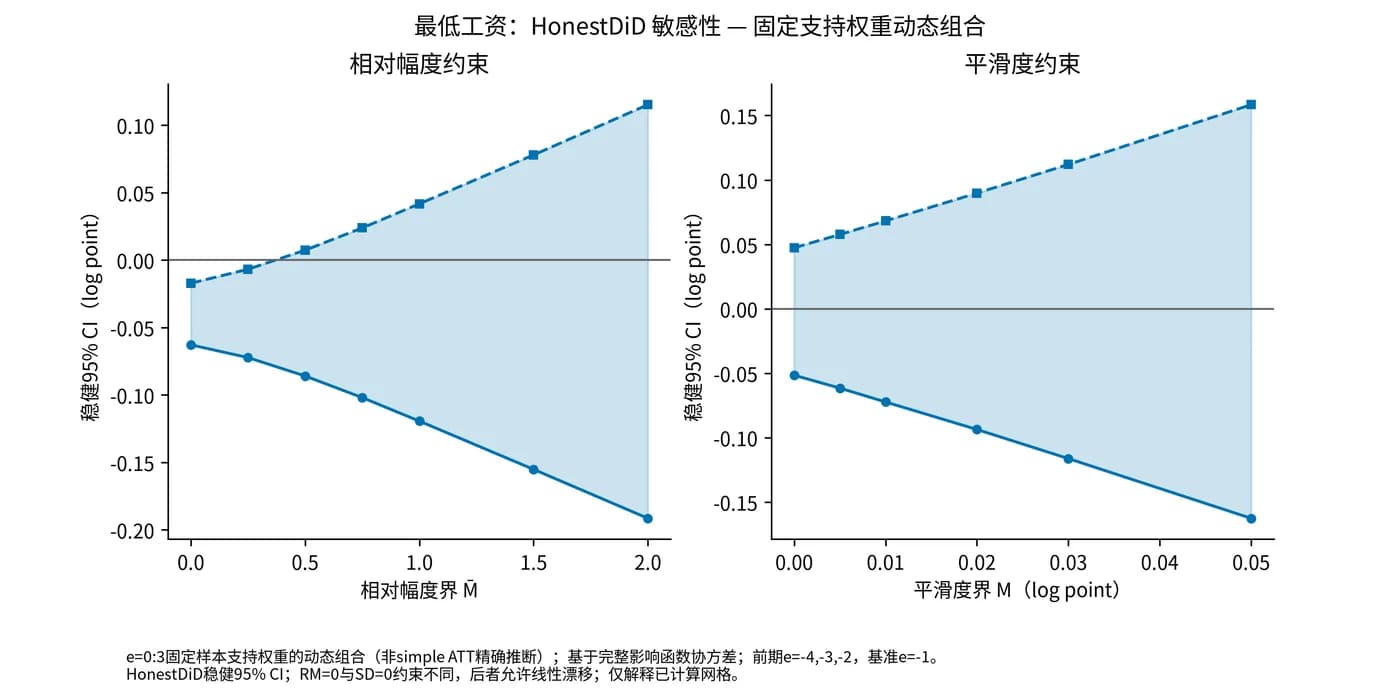
Choose by your situation
Why this stepCallaway–Sant'Anna allows two kinds of control group. The choice depends on whether enough units are never treated and whether you accept a no-anticipation assumption.
Use never-treated controls when enough units are never treated and they are not very different from the treated. mpdta has 309 never-treated counties and the castle data have 29 states. Not-yet-treated controls also use units that have not been treated yet. The sample is larger, but you must assume there is no anticipation before treatment.
On these data the two choices differ very little: the simple overall effect for mpdta is -0.0400 and -0.0398, and for the castle data 0.1104 and 0.1094. A careful comparison matters when few units are never treated or when they differ a lot from the treated.
Why this stepCovariates relax parallel trends into conditional parallel trends: units with the same characteristics share the same trend. TWFE and Callaway–Sant'Anna handle covariates differently.
Covariates that do not vary over time are absorbed by the unit fixed effects. After adding baseline lpop to mpdta the TWFE coefficient stays at -0.0365, while the Callaway–Sant'Anna overall effect (doubly robust, never treated) moves from -0.0400 to -0.0418 and its standard error falls from 0.0122 to 0.0113.
Covariates need overlap between treated and control units. When baseline income, unemployment and poverty were added to the castle data, the 2009 cohort has a single state and the estimation reports overlap condition violated. Do not drop the failed cohort. Report it as it is and add outcome regression, which does not rely on propensity scores, as a supplement.
Why this stepEvery estimator here has a Stata command. Use R when you have no Stata license or want reproducible scripts.
The R package and the Stata command for an estimator implement the same paper, so point estimates should agree in principle. Bootstrap standard errors and the default base period can differ. The did package defaults to a base period that moves with the comparison (varying), while this page uses universal, so align the settings before comparing.
| Method | R package and function | Stata command |
|---|---|---|
| Callaway–Sant'Anna | did::att_gt, aggte | csdid |
| Goodman-Bacon decomposition | bacondecomp::bacon | bacondecomp |
| Sun–Abraham | fixest::sunab | eventstudyinteract |
| BJS imputation | didimputation::did_imputation | did_imputation |
| HonestDiD | HonestDiD | honestdid |
| TWFE | fixest::feols | reghdfe |
Why this stepThe numbers on this page come from one run in which a Scientify agent worked from a written task brief. You can reuse the brief for your own project.
The brief states the research question, the data, the software, the required tests, the literature to check and the deliverables. The agent installed packages on the cloud computer, ran the estimates, checked literature values, and produced a 15-page Chinese report, a results workbook and reproducible scripts in 33 minutes without renting external compute.
The agent found three limitations on its own and wrote them into the report. First, the minimum wage result depends on the earliest cohort: dropping the 20 counties of the 2004 cohort changes the Callaway–Sant'Anna overall effect from -0.0400 to -0.0249. Second, the covariate model for the castle data lacks overlap in the 2009 cohort. Third, the paywalled Cheng–Hoekstra pages could not be opened, so it quoted only the roughly 8% in the abstract and marked the table coefficients as unverified.
Concepts and judgment
Why this stepWith two periods and two groups TWFE is the ordinary DiD. With staggered timing it becomes a weighted average of several 2×2 comparisons whose weights depend on cohort sizes and timing.
When the treatment effect is the same across cohorts and periods, this weighted average is still correct. When the effect changes with time since treatment or differs across cohorts, comparisons that use already-treated groups as controls bring the control group's own effect into the estimate. The result can drift from the true average effect and even flip sign (Goodman-Bacon, 2021).
How large the bias is depends on the weight of those comparisons and on how much the effect varies. In the two datasets here those comparisons carry only 5.4% and 3.2% of the weight, and the gap between TWFE and the newer estimators is within the standard errors. Not every dataset will behave this way, so run the decomposition on your own data.
Why this stepNo. Bacon weights only describe the share of each 2×2 comparison in TWFE. They cannot explain all of the gap between TWFE and the newer estimators.
In the castle data TWFE is 0.0818 and Callaway–Sant'Anna is 0.1104, a gap of 0.0286. The comparisons that use already-treated controls contribute only 0.0022 to TWFE. The treated-versus-never-treated comparisons average 0.0880, still below 0.1104. Part of the remaining gap comes from the different ways TWFE and Callaway–Sant'Anna weight cohorts and periods.
Report TWFE together with at least one robust estimator and state their aggregation target and weights. When the two are close, the conclusion is not sensitive to the estimator. When they differ, look at the decomposition and weights first, then at whether the effect changes over time.
Reference and appendix
Why this stepThe table lists the comparisons that could be verified. Values that could not be verified are not in it.
The mpdta data in did is a subset of the paper's data, a different sample from Table 3, so values cannot match one for one. The TWFE value of -0.0365 is close to the paper's -0.037, while the simple and event-study overall effects are smaller than the paper's. The dynamic overall effect and ATT(g,t) match the official did documentation, which shows the workflow here agrees with the official one on the same data.
The abstract of Cheng and Hoekstra (2013) reports a statistically significant 8 percent net increase in homicides. The TWFE value of 0.0818 here is of similar size, but this page does not use the paper's population weights and controls, its standard error is 0.0589, and it is not significant. The paper's significance is not reproduced.
| Source | Quantity | Literature (SE) | This page (SE) |
|---|---|---|---|
| CS 2021 paper, Table 3(a) | TWFE | -0.037 (0.006) | -0.0365 (0.0133) |
| CS 2021 paper, Table 3(a) | Simple weighted average | -0.052 (0.006) | -0.0400 (0.0122) |
| CS 2021 paper, Table 3(a) | Event study | -0.090 (0.013) | -0.0772 (0.0203) |
| did documentation | Dynamic overall ATT | -0.0772 (0.0203) | -0.0772 (0.0203) |
| did documentation | ATT(2004, 2004 to 2007) | -0.0105、-0.0704、-0.1373、-0.1008 | -0.0105、-0.0704、-0.1373、-0.1008 |
| Cheng–Hoekstra 2013 abstract | Net increase in homicides | about 8%, significant | 0.0818 (0.0589) |
Why this stepThe environment, timing and verification.
On 2026-11-06 a Scientify agent completed the whole analysis from the brief on a standard-tier cloud computer (2 CPU cores) in 33 minutes. The versions were R 4.4.3, did 2.5.1, fixest 0.14.2, bacondecomp 0.1.1, didimputation 0.5.1 and HonestDiD 0.2.8. The random seed was 20261106 with 999 multiplier-bootstrap draws.
On 2026-11-09, with intermediate results cleared on a different cloud computer, the agent's full scripts reproduced the TWFE, Callaway–Sant'Anna, Bacon weights, HonestDiD intervals and permutation p-value of the original run. The compact scripts downloadable here ran on the same machine: a few seconds for each estimation script and about a minute for the HonestDiD script. The only difference is the Castle Callaway–Sant'Anna standard error, which depends on the bootstrap draws (0.0420 and 0.0397).
Troubleshooting by error or symptom
Every error below appeared in the runs for this page.
overlap condition violated for group 2009
Cause: After covariates are added, a cohort has too few units to estimate propensity scores. The 2009 cohort here has a single state.
Fix: Keep the failed cohort and its NA instead of dropping it to make the code run. Report the result without covariates and add outcome regression on the same covariates (est_method = "reg") as a supplement.
Missing values found in att_gt() estimates
Cause: A consequence of the previous item: the failed cohort has NA in ATT(g,t) and aggte meets missing values.
Fix: The aggregate covers only the identifiable cohorts. State in the report which cohorts are missing.
Not returning pre-test Wald statistic due to singular covariance matrix
Cause: The covariance matrix of the pre-test is singular, which tends to happen in panels with many pre-treatment coefficients and cohorts of a single state. It appears when running att_gt on the castle data.
Fix: Do not report the missing Wald statistic as a pass. Test the identifiable pre-treatment coefficients at the event-time level instead, for example e = -4 to -2 (p = 0.186 here), and note that the far leads have little data.
Some groups in your dataset have very few observations, which may cause estimation problems
Cause: Some treatment cohorts have only one or two units. The 2005, 2007, 2008 and 2009 cohorts in the castle data triggered the warning.
Fix: This is a warning and the run continues. ATT(g,t) for small cohorts is very imprecise, so read single-cohort results with their confidence intervals and state in the limitations how much the aggregate depends on them.
Installing HonestDiD fails with The 'rustc' compiler was not found on the PATH
Cause: HonestDiD depends on CVXR, CVXR depends on clarabel, and clarabel builds from source and needs Rust (rustc 1.70 or newer). The cloud computer image has no Rust toolchain, and the first install took 649 seconds before it reported this error.
Fix: Install Rust first, then clarabel and HonestDiD. The agent installed rustup (minimal profile) inside the workspace and set MAKEFLAGS=-j1 and CARGO_BUILD_JOBS=1 to limit memory use. The follow-up install took about 147 seconds.
export MAKEFLAGS=-j1 CARGO_BUILD_JOBS=1
Rscript -e 'install.packages("HonestDiD")'
The estimation was done without fixed-effects (FE). The FE coefficients cannot be retrieved.
Cause: A time-invariant covariate (baseline lpop in mpdta) was added to the first stage of did_imputation and is collinear with the unit fixed effects.
Fix: Write the first stage as ~ 0 | unit + year only. Time-invariant covariates are already absorbed by the unit fixed effects.
Error: all(complete.cases(d)) is not TRUE
Cause: A data-integrity check treated the generated event-time variable, which is NA for never-treated units, as missing data.
Fix: Run the completeness check on the original columns only, for example complete.cases(mpdta), and not on generated columns.
Sources
- Callaway, B., Sant'Anna, P. H. C. (2021). Difference-in-Differences with multiple time periods. Journal of Econometrics. — The Callaway–Sant'Anna estimator; Table 3 from arXiv 1803.09015
- Goodman-Bacon, A. (2021). Difference-in-differences with variation in treatment timing. Journal of Econometrics. — The Bacon decomposition
- Sun, L., Abraham, S. (2021). Estimating dynamic treatment effects in event studies with heterogeneous treatment effects. Journal of Econometrics. — The Sun–Abraham estimator
- Borusyak, K., Jaravel, X., Spiess, J. (2024). Revisiting Event-Study Designs: Robust and Efficient Estimation. Review of Economic Studies. — BJS imputation estimator
- Rambachan, A., Roth, J. (2023). A More Credible Approach to Parallel Trends. Review of Economic Studies. — The HonestDiD method
- Baker, A. C., Larcker, D. F., Wang, C. C. Y. (2022). How much should we trust staggered difference-in-differences estimates? Journal of Financial Economics. — Simulation evidence on TWFE under staggered treatment
- Cheng, C., Hoekstra, M. (2013). Does Strengthening Self-Defense Law Deter Crime or Escalate Violence? Journal of Human Resources. — The original study behind the castle doctrine data; only the abstract is quoted here
- did package documentation: Getting started with the did package — Page dated 2026-07-30, did 2.5.1; description of mpdta and reference ATT(g,t) values
- Cunningham, S. Causal Inference: The Mixtape, castle.dta — Download source of the castle data