 Scientify
About this page
Tutorial- What this page solves
- You want to write an association study with NHANES but are unsure where to download files, which weight to use, how to link mortality, and how to run Cox and RCS models correctly.
- Who it is for
- Medical graduate students and clinicians working with public databases. You should know R and the basics of Cox regression.
- What you will have
- A complete NHANES mortality workflow, what each step should produce, and a real set of results to compare against.
- Covers
- Download paths and variable lookup for official NHANES files
- Parsing the fixed-width NCHS mortality file and defining cardiovascular death
- Choosing fasting subsample weights and multi-cycle factors
- The TyG formula and unit conversion
- Survey-weighted Cox regression, RCS curves and weighted Kaplan-Meier curves
- Subgroup interactions, proportional hazards checks and sensitivity analyses, with real results
- Does not cover
- Two-day dietary weights for 24-hour recalls
- Causal inference methods such as Mendelian randomization
- Writing the introduction and discussion
Main path: step by step
Step 1
Why this stepEach module in each NHANES cycle is a separate XPT file, so first decide which files you need.
The official entry point is wwwn.cdc.gov/nchs/nhanes. Data are released in two-year cycles since 1999, and each cycle has five module groups: demographics, dietary, examination, laboratory and questionnaire, each with several XPT files. Choose a cycle and a module on the site to see the file list and variable documentation (Doc File).
NHANES is run by NCHS, part of the US CDC. Since 1999 it has been released in two-year cycles, free of charge. File names carry a letter suffix per cycle: none for 1999–2000, _B for 2001–2002, through _J for 2017–2018. All files merge on the participant ID SEQN.
This example downloaded 100 official files across ten cycles. CDC has changed its download paths: the old path /Nchs/Nhanes/2017-2018/DEMO_J.XPT now returns an HTML 404 page. Use the new path, and check the start of each file to confirm it is XPT data rather than an error page.
https://wwwn.cdc.gov/Nchs/Data/Nhanes/Public/2017/DataFiles/DEMO_J.xpt
# the year is the first year of the cycle; the file name carries the cycle suffixlibrary(haven)
demo <- read_xpt("DEMO_J.xpt")
glu <- read_xpt("GLU_J.xpt")
trig <- read_xpt("TRIGLY_J.xpt")
d <- Reduce(function(x, y) merge(x, y, by = "SEQN", all.x = TRUE), list(demo, glu, trig))| Cycle | Demographics | Fasting glucose | Triglycerides |
|---|---|---|---|
| 1999–2000 | DEMO | LAB10AM | LAB13AM |
| 2001–2002 | DEMO_B | L10AM_B | L13AM_B |
| 2003–2004 | DEMO_C | L10AM_C | L13AM_C |
| 2005–2006 | DEMO_D | GLU_D | TRIGLY_D |
| 2007–2018 | DEMO_E … DEMO_J | GLU_E … GLU_J | TRIGLY_E … TRIGLY_J |
Step 2
Why this stepMortality outcomes come from public files that NCHS releases after linking NHANES to the National Death Index (NDI).
This example uses the 2019 public-use linked mortality files, one .dat file per cycle. They are fixed-width and must be read with the column positions from the official NCHS read program, not as CSV.
Cardiovascular death is UCOD_LEADING equal to 001 (heart disease) or 005 (cerebrovascular disease). Follow-up time is PERMTH_EXM, months from the examination to death or the end of follow-up. Check cause-of-death code frequencies and the follow-up range after reading.
https://ftp.cdc.gov/pub/Health_Statistics/NCHS/datalinkage/linked_mortality/NHANES_2017_2018_MORT_2019_PUBLIC.dat| Variable | Columns | Meaning |
|---|---|---|
| SEQN | 1–6 | Participant ID |
| ELIGSTAT | 15 | Linkage eligibility, 1 = eligible |
| MORTSTAT | 16 | Vital status, 1 = deceased |
| UCOD_LEADING | 17–19 | Leading underlying cause of death |
| PERMTH_INT | 43–45 | Months of follow-up from interview |
| PERMTH_EXM | 46–48 | Months of follow-up from examination |
Step 3
Why this stepNHANES is a complex survey. Unweighted results describe the sample, not the US population.
The rule is that the variable from the smallest subsample determines the weight. Fasting glucose and triglycerides are measured only in the morning fasting subsample, so a TyG study must use the fasting weight (WTSAF2YR, or WTSAF4YR for 1999–2002), not the examination weight WTMEC2YR.
When combining cycles, multiply each cycle's weight by its years over the total years. Here 20 years are combined: the four-year 1999–2002 weight is multiplied by 4/20 and each two-year weight from 2003 onward by 2/20. The design variables SDMVPSU (PSU) and SDMVSTRA (stratum) are in the DEMO files.
library(survey)
d$wt20 <- ifelse(d$cycle %in% c("1999-2000", "2001-2002"),
                 d$WTSAF4YR * 4 / 20,
                 d$WTSAF2YR * 2 / 20)
options(survey.lonely.psu = "adjust")
des <- svydesign(ids = ~SDMVPSU, strata = ~SDMVSTRA,
                 weights = ~wt20, nest = TRUE, data = d)
# build the design on the full sample, then subset(); do not drop rows first
des_a <- subset(des, analysis_flag == 1)Step 4
Why this stepDefine the exposure and the final analysis sample.
NHANES LBXTR and LBXGLU are already in mg/dL; use them directly without converting again. Inclusion criteria: age ≥20, not pregnant, positive fasting glucose and triglycerides, fasting weight above 0, eligible for mortality linkage, and follow-up after the examination above 0.
TyG = ln[ TG (mg/dL) × FPG (mg/dL) / 2 ]

# if values are in mmol/L, convert first: TG × 88.57, glucose × 18.018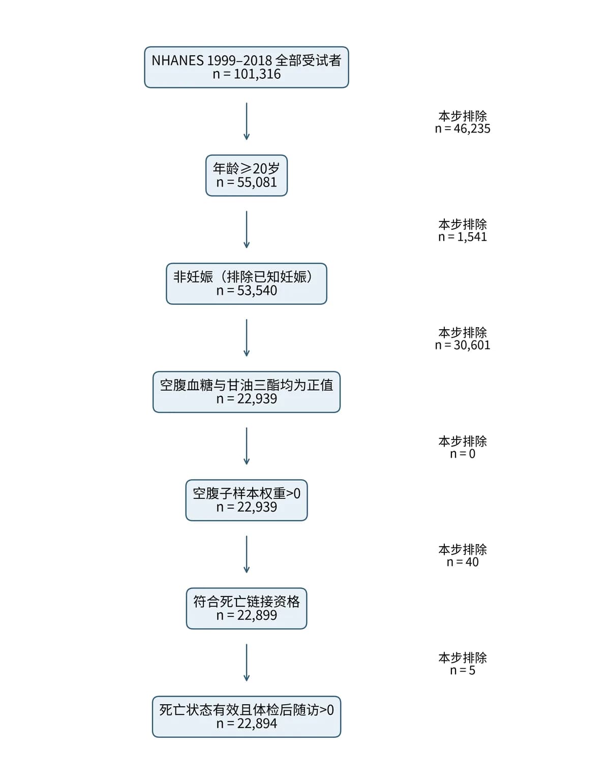
Step 5
Why this stepEstimate how mortality risk changes per one-unit increase in TyG.
After full adjustment the linear HR confidence interval crosses 1. A non-significant linear term does not mean no association, so the next step checks for a nonlinear relationship with RCS. When the 95% CI crosses 1, do not claim a statistical association.
fit <- svycoxph(Surv(PERMTH_EXM, MORTSTAT) ~ tyg + age + sex + race +
                  edu + pir + smoke + bmi + diabetes + hypertension +
                  cvd + cancer, design = des_a)
summary(fit)| Outcome | Model 3: HR per 1 unit TyG (95% CI) |
|---|---|
| All-cause mortality | 1.03 (0.95–1.12) |
| Cardiovascular mortality | 1.10 (0.93–1.29) |
Step 6
Why this stepRCS does not assume linearity and tests whether the exposure–outcome relationship is curved.
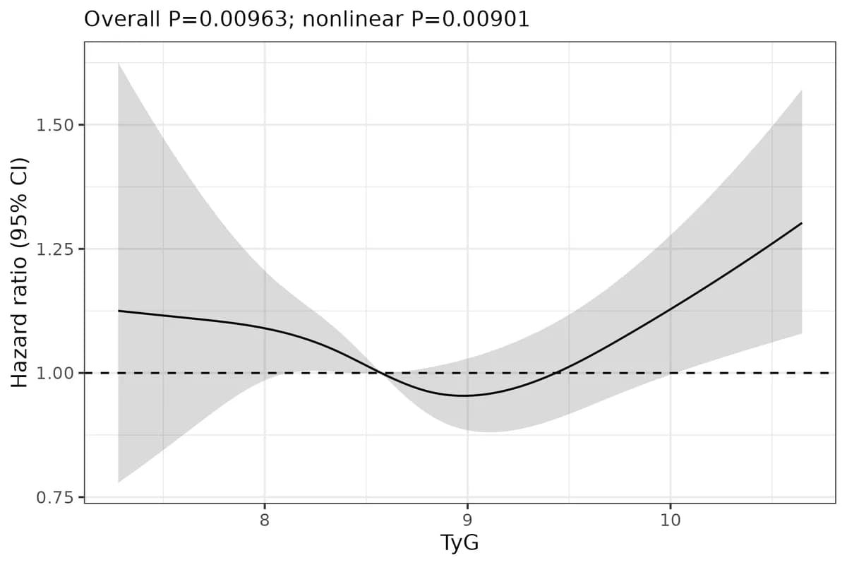
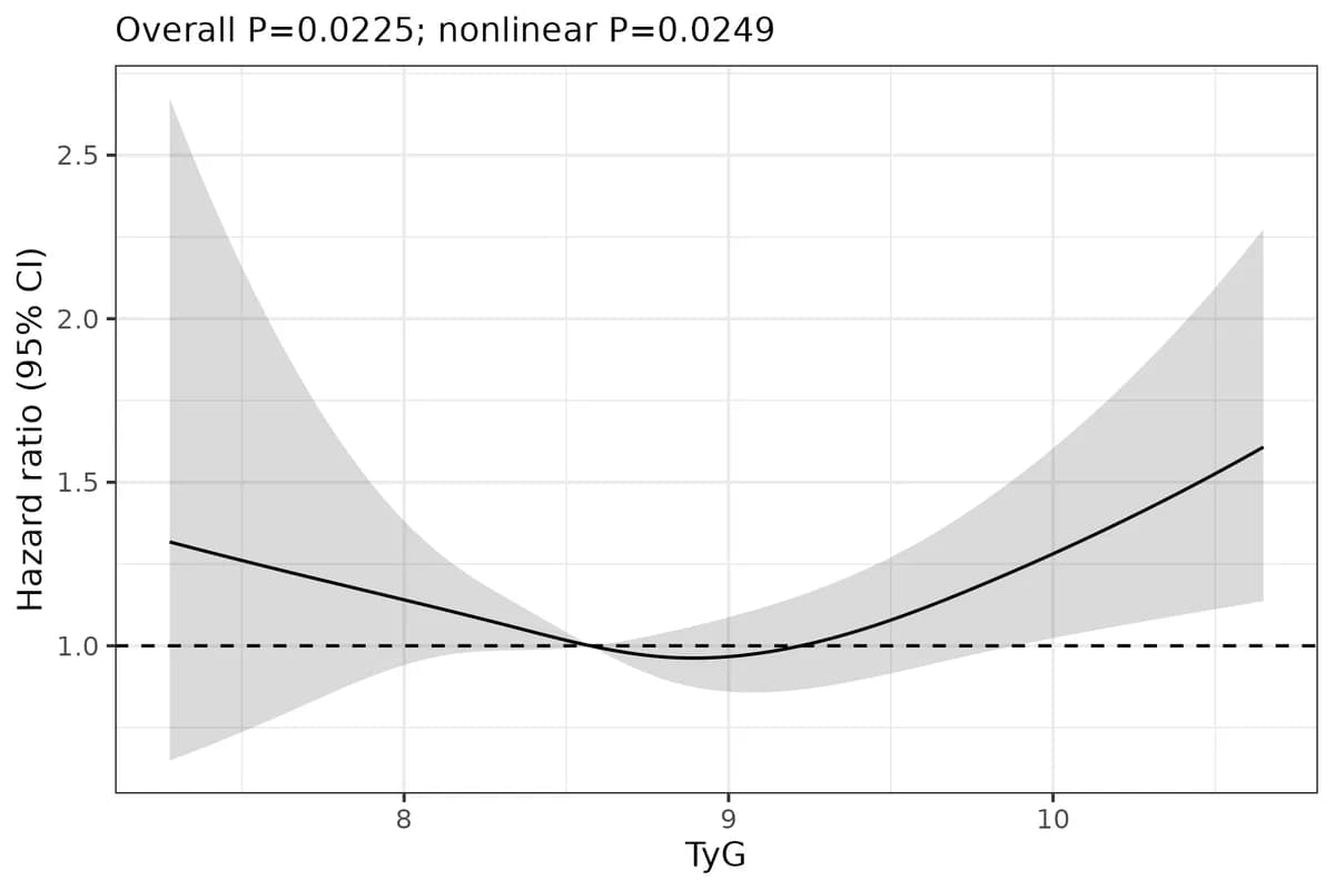
This example uses 4 knots in the weighted Cox model at the 5th, 35th, 65th and 95th weighted percentiles of TyG (7.63, 8.33, 8.82, 9.76), with the weighted median 8.57 as reference. RCS gives two P values: the overall P tests any association, and the nonlinear P tests departure from a straight line.
For all-cause mortality the overall P is 0.0096 and the nonlinear P is 0.0090. The curve is U-shaped with its lowest point near TyG 9.0. For cardiovascular mortality the nonlinear P is 0.025.
Step 7
Why this stepCox models assume the HR does not change over time, which needs checking. KM curves show survival by group.
Calling cox.zph directly on an svycoxph fit gives P values near 1. This is an artefact of the weight scale and the test should not be used. Here follow-up was split into 0–60, 60–120 and >120 months, and a TyG × period interaction was tested with a design-based Wald test: P = 0.034 for all-cause mortality, which suggests non-proportional hazards, so period-specific HRs are also reported; P = 0.49 for cardiovascular mortality.
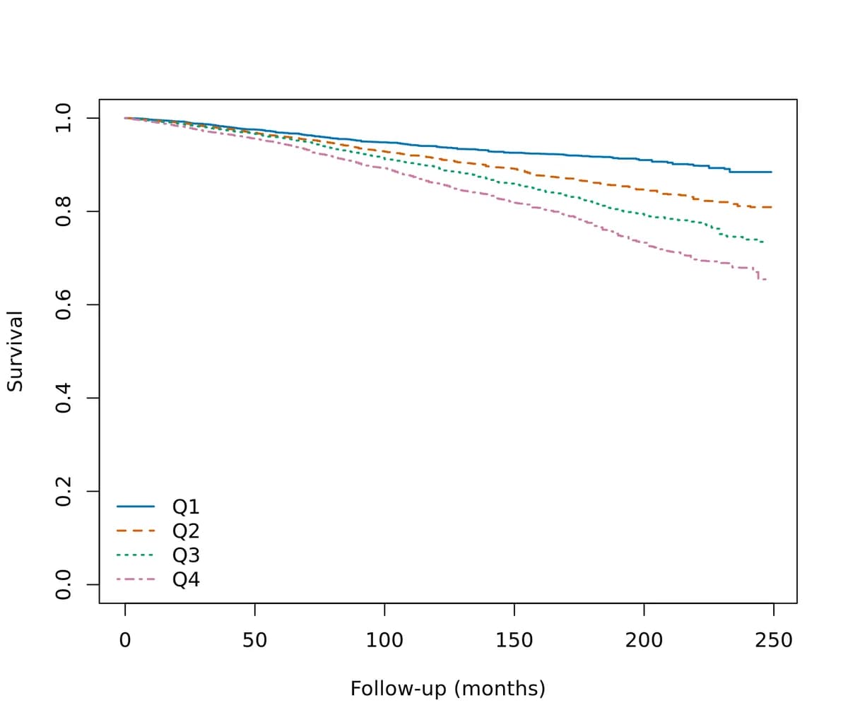
Weighted KM curves by TyG quartile use survey::svykm, with group comparison by survey::svylogrank. Curves labeled as weighted must be weighted estimates.
Step 8
Why this stepTest whether the TyG–mortality association differs across populations.
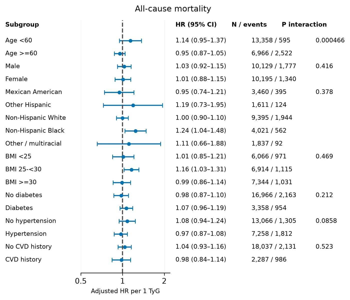
Seven subgroups were prespecified: age (<60 / ≥60), sex, race, BMI, diabetes, hypertension and cardiovascular history. Each stratum reports HR, 95% CI, participants and events, with an interaction P value. Only the age interaction was significant (P < 0.001): HR 1.14 (0.95–1.37) under 60 and 0.95 (0.87–1.05) at 60 or older.
Judge subgroup differences by the interaction P value, not by one stratum being significant and another not. Here the non-Hispanic Black stratum has HR 1.24 (1.04–1.48), but the race interaction P is 0.378, so it is wrong to say TyG matters only in that group. Subgroup tests were not corrected for multiple comparisons and are exploratory.
Step 9
Why this stepCheck whether the main conclusion holds under other reasonable choices.
| Analysis | Purpose |
|---|---|
| Exclude deaths in the first 2 years | Reduce reverse causation from baseline illness |
| Exclude baseline cardiovascular disease and cancer | Reduce the influence of existing disease |
| Multiple imputation (m = 5, 10 iterations) | Handle missing covariates; outcome, follow-up, exposure, weights and strata enter the imputation model, pooled with Rubin's rules |
| Unweighted Cox | Show the effect of weighting |
Concepts and judgment
Comparison
Why this stepWhy studies using the same database and index reach different numbers.
The shared finding is a non-significant quartile trend test together with a nonlinear RCS. These do not conflict: the trend test checks monotonic change, while RCS allows curvature. Inflection points depend on age structure and covariates, so 8.88, 9.18 and 9.364 should not be used as clinical cut-offs.
| Study | Sample | Main result |
|---|---|---|
| Chen et al., 2024 | 1999–2018, n = 17,118 | All-cause Q4 vs Q1 HR 0.93 (0.76–1.14); RCS threshold 8.88, nonlinear P = 0.0071 |
| Wang et al., 2024 | 2001–2018, n = 15,388 | All-cause Q4 HR 1.02 (0.62–1.48); curve falls then rises |
| Sun et al., 2022 | 1999–2014, age ≥45, n = 9,254 | All-cause continuous HR 1.01 (0.93–1.10); inflection point 9.18 |
| This page | 1999–2018, age ≥20, n = 22,894 | All-cause continuous HR 1.03 (0.95–1.12); U-shaped, minimum near 9.0, exploratory breakpoint 9.364 |
Reference and appendix
Run record
Why this stepData source and run conditions.
The numbers come from one long research task on Scientify on 27 October 2026. After the user uploaded a task brief and confirmed six research requirements, Scientify downloaded 100 official files, parsed the mortality files, combined weights and ran every analysis. It also caught the weight-scale artefact of cox.zph on a weighted model and switched to a time-interaction test.
The deliverables were a 16-page report in Chinese, 22 figures, tables, a one-command reproduction script and a data manifest with SHA256 hashes, and an independent review passed. The task took about 1.5 hours on a cloud CPU without renting a GPU.


Common errors and fixes
Ordered by how often they occur.
WTMEC2YR used for a fasting-laboratory analysis
Cause: Fasting glucose and triglycerides are measured only in the fasting subsample.
Fix: Use WTSAF2YR (WTSAF4YR for 1999–2002) and rescale by cycle years when combining.
Downloaded XPT files cannot be read, or are only a few KB
Cause: CDC changed its paths and the old URLs return an HTML 404 page.
Fix: Use /Nchs/Data/Nhanes/Public/<year>/DataFiles/ and check the file header after download.
Weighted standard errors are unusually small
Cause: Rows were dropped before svydesign, which breaks the sampling structure.
Fix: Build the design on the full sample, then use subset().
Mortality columns are misaligned
Cause: The fixed-width .dat file was read as delimited text.
Fix: Use the column positions from the official NCHS read program; SEQN is columns 1–6.
TyG values are clearly too large
Cause: mg/dL values were multiplied by a conversion factor again.
Fix: LBXTR and LBXGLU are already mg/dL; use them directly.
cox.zph on svycoxph gives P values near 1
Cause: An artefact of the weight scale; the test is invalid.
Fix: Use a time-period interaction with a design-based Wald test.
survey reports a lonely PSU error
Cause: A stratum in the subset has only one PSU.
Fix: Set options(survey.lonely.psu = "adjust") and state it in the methods.
References
- NHANES data portal (CDC)
- NHANES weighting tutorial (NCHS) — Rules for combining cycles
- NCHS public-use linked mortality files — Includes official read programs
- Chen et al., Lipids in Health and Disease 2024
- Wang et al., Frontiers in Endocrinology 2024
- Sun et al., BMC Geriatrics 2022